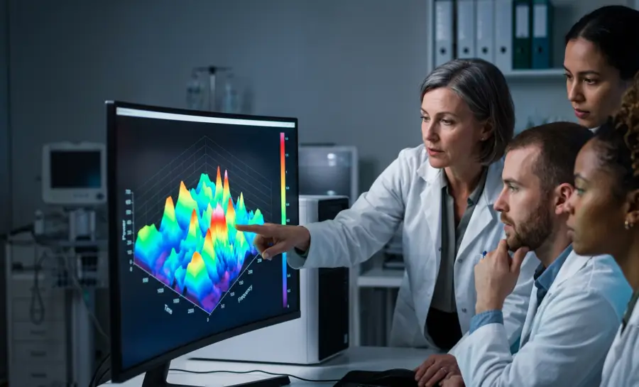
Discrete fourier analysis (DFT) provides a robust framework for deconstructing complex signals into their fundamental periodic components for precise interpretation.
This article works through how the DFT converts a finite block of sampled voltage data, such as a resting-state recording or a single block from a task-based experiment, into a set of frequency components.
What Is Discrete Fourier Analysis?
Discrete fourier analysis is a mathematical approach used to interpret sampled signals by decomposing them into a series of constituent frequencies.
Instead of viewing data as a continuous flow, this method processes discrete, finite sequences of numbers—such as voltage readings from EEG recording systems—to identify the relative strengths of various oscillation cycles. By converting these samples into numerical representations of amplitude and phase, researchers gain a clear perspective on which frequency components are most dominant within a dataset.
This technique bridges the gap between raw data collection and meaningful information extraction, functioning essentially as a digital prism. When applied to complex waveforms, the process separates overlapping oscillations into readable bands, allowing for the isolation of specific rhythmic signatures that would otherwise remain masked by broader signal noise. It is a cornerstone of modern neuroscience research, where isolating distinct brain activity patterns is essential for understanding both healthy neural function and pathological states.
By leveraging the ability of frequency analysis to reorganize temporal sequences, scientists can effectively filter out ambient electrical noise or artifacts that might contaminate a reading. This transformation is not merely a statistical exercise but a vital tool that makes subtle, high-frequency oscillations visible in a quantitative format. The resulting distribution of power across different frequency bands forms the basis for much of the diagnostic assessment performed in contemporary clinical labs today.
What the Discrete Fourier Transform (and FFT) Actually Do in EEG Signal Processing
Once a continuous EEG signal has been sampled into a finite sequence of numbers, the DFT can operate on it. Given N samples of voltage, the DFT produces N complex numbers, each one representing the contribution of a specific, narrow slice of frequency, referred to as a bin. Instead of one messy voltage trace, you end up with a structured list showing how much of each frequency is present in that recording.
Computing a DFT directly becomes slow as N grows large, since the calculation scales with the square of the number of samples. The fast Fourier transform, or FFT, is an algorithm that produces mathematically identical results while running far more efficiently.
In practice, virtually nobody computes a raw DFT by brute force. The FFT is simply the standard, efficient way of getting there, and the two terms are often used interchangeably in EEG research.
How to Read a Raw EEG Frequency Spectrum
Suppose a recording contains N samples, taken at a sampling rate of fₛ samples per second. The DFT of that recording produces N evenly spaced frequency bins spanning from 0 Hz up to fₛ Hz.
The spacing between adjacent bins, called the bin width, equals fₛ divided by N. This single number, the bin width, determines the finest frequency detail the analysis can distinguish.
Because EEG voltage is a real-valued signal rather than a complex one, only the first half of these bins, specifically N/2 + 1 of them, contain unique information. The remaining bins are mirror images of the first half and add nothing new. Bin number k corresponds to a real frequency of k multiplied by the bin width (fₛ / N).
At each of these bins, the DFT outputs a complex number, meaning it has two components rather than one. The magnitude of that complex number is the amplitude of the corresponding frequency component, expressed in microvolts once properly scaled. This tells you how strong that particular rhythm is within the recorded segment.
The angle of the complex number is the phase, which tells you where in its cycle that rhythm happens to be at the start of the recording, effectively marking when the rhythm peaks relative to the beginning of the window.
Three Constraints That Shape Every EEG Spectrum
Three practical limits govern how trustworthy a DFT-based spectrum actually is, and all three trace back to the fact that the input is a finite, sampled record rather than an infinite, continuous one:
Bin width (frequency resolution) equals fₛ divided by N; only a longer recording can separate two nearby rhythms.
Nyquist limit at half the sampling rate permanently aliases faster brain activity unless filtered before sampling.
Spectral leakage spreads a rhythm’s energy into neighboring bins when its frequency falls between bin centers; tapering windows reduce the spread.
Applying the DFT to Resting-State and Block-Design EEG
The DFT assumes, at least implicitly, that the frequency content of the signal does not shift much during the segment being analyzed. This assumption is reasonable during sustained rest or a uniform block of a repetitive cognitive task, states that are approximately stationary. In those conditions, a single DFT taken across the whole epoch produces a spectrum that meaningfully represents the brain's rhythmic activity for that stretch of time.
This is close to the approach used in a legacy study of hemispheric EEG asymmetry, where participants performed verbal, arithmetic, spatial, and musical tasks while EEG was recorded from temporal and parietal electrode sites.
Discrete Fourier transforms of these recordings produced power ratios comparing the right and left hemispheres across standard frequency bands. The alpha band showed that asymmetry between hemispheres depended significantly on which task was being performed, and the hemisphere more actively engaged by the task consistently showed proportionately less alpha power.
This task-dependent effect in the alpha band was reported as 2 to 5 times larger than what earlier research had found when looking at whole-band power without isolating alpha specifically. That gain in sensitivity came directly from separating frequency bands with the DFT rather than treating the signal as one undivided block.
Moreover, a study from the Fukui University of Technology in Japan of normal and epileptic EEG offers a similar pattern applied to likely resting-state conditions. Its Fourier analysis revealed the 1/f-like spectral shape mentioned earlier and confirmed that the alpha rhythm, prominent in the normal recordings, was absent from the epileptic ones.
Limitations: When the DFT Falls Short
The DFT's core assumption, that frequency content stays constant across the analyzed segment, breaks down whenever EEG activity changes rapidly within that window. Epileptic spikes and sudden emotional shifts are two clear examples of this kind of non-stationary behavior.
The study analyzing normal and epileptic EEG demonstrated this limitation directly. While the Fourier transform successfully captured the overall 1/f spectral shape of the recordings, it failed to reveal the localized spikes and sharp complexes typical of seizure activity.
Wavelet transforms, a different family of time-frequency tools, were able to detect those localized events where the Fourier approach could not.
The practical conclusion is straightforward: for stationary recordings, resting-state blocks or well-controlled task blocks, the DFT provides a solid and interpretable foundation for frequency analysis. For transient or rapidly shifting events, time-frequency extensions such as wavelets or adaptive short-time transforms may be necessary.
Discrete Fourier Analysis and Wavelets: How They Compare
Discrete fourier analysis provides an excellent global view of a signal, identifying the static frequency composition over an entire block of data. Because it calculates a single average spectrum for that time window, it is highly efficient for stationary signals where the rhythmic properties remain consistent. However, it lacks the ability to resolve precisely when a specific frequency event occurs within that analyzed segment, essentially blurring temporal features into a single aggregate portrait.
In contrast, wavelets offer a multiresolution approach that provides localized information in both time and frequency. By utilizing a window that varies in size, wavelet transforms can zoom in on transient spikes or sudden bursts of activity, which are often lost when using broader Fourier methods. This makes them significantly more flexible for examining episodic brain phenomena or rapid neurological shifts that do not follow a set periodic pattern.
Choosing between these methods is a matter of prioritizing information needs within the research project parameters. Researchers often follow a standard procedural workflow for determining their signal processing strategy:
Confirm if the signal of interest is stationary or transient.
Apply traditional global spectral analysis for mean power assessment.
Implement time-frequency decomposition for localized event tracking.
Validate the resulting energy distributions against known physiological artifacts.
Discrete Fourier Analysis Python Implementation Guide
Implementing this analysis in Python typically involves the use of specialized libraries like NumPy or SciPy, which provide optimized functions for computing fast Fourier transforms.
The primary function fft accepts an array of voltage samples and returns a complex-valued container representing the power and phase at each harmonic. Developers must ensure the input array is correctly padded if necessary, though modern libraries handle the underlying matrix operations automatically for most standard array sizes.
After computing the raw transform, the real-world implementation requires normalization of the output and the absolute value calculation to derive the power spectrum. This involves dividing by the total length of the sequence to scale the magnitudes appropriately. Once scaled, the spectrum can be plotted against a defined frequency axis, which is constructed based on the original sampling frequency of the recording hardware.
Finalizing the code requires handling potential artifacts by cleaning the incoming signal first through bandpass filters. By isolating only the frequencies of interest to the current study, users reduce the computational footprint and improve the interpretability of the final spectral graph. This modular approach allows for rapid refinement of processing pipelines as new research requirements emerge.
Discrete Fourier Analysis PDF Guides and Resources
For those seeking deep technical manuals, there are several foundational PDF resources that detail the mathematical proofs and implementation strategies for spectral analysis. These documents serve as a bridge between theoretical signal processing textbooks and practical lab applications, clarifying how to account for error bounds and system-specific biases. Many of these guides are curated by academic research groups for the purpose of standardizing processing across multi-institutional studies.
These resources frequently include tutorials on preparing raw time-series data for analysis, emphasizing specific data cleanliness requirements such as artifact rejection and re-referencing. They also provide comprehensive overviews of various windowing functions, explaining how they influence the trade-off between spectral resolution and amplitude accuracy. Understanding these nuances is essential for any practitioner looking to move beyond black-box implementations of common library functions.
By consulting these technical guides, students and researchers can gain insight into the common pitfalls associated with digital transformations, such as spectral leakage and wrap-around artifacts. These guides are periodically updated to reflect advancements in computational speed and efficiency, ensuring that the methodologies described remain current and applicable to modern high-resolution sampling hardware used in current scientific projects.
How Frequency Analysis Reveals Hidden Brain Rhythms
Breaking an EEG recording into its component frequencies turns a tangled voltage trace into something far more telling. The discrete Fourier transform shows exactly which rhythms are present and how strong they are, which is why it has become the first step in extracting features like alpha-band asymmetry linked to mental tasks or the distinct 1/f shape that separates normal brain activity from epileptic recordings. This step provides a clear, interpretable picture of the brain's oscillatory landscape during stable, resting or task-based states.
However, the method carries important boundaries as it needs a fast enough sampling rate to avoid aliasing, a long enough window to tell close rhythms apart, and an awareness that sudden neural events break its core assumption of a steady brain state. For those transient spikes or rapid emotional shifts, researchers often turn to time-frequency alternatives, though comparisons of these tools across many tasks remain sparse.
Understanding what the raw amplitude spectrum can and cannot say keeps the focus on what the data actually support, building a careful picture of brain function study by study.
References
Doyle, J. C., Ornstein, R., & Galin, D. (1974). Lateral specialization of cognitive mode: II. EEG frequency analysis. Psychophysiology, 11(5), 567-578. https://doi.org/10.1111/j.1469-8986.1974.tb01116.x
Yamaguchi, C. (2003, March). Fourier and wavelet analyses of normal and epileptic electroencephalogram (EEG). In First International IEEE EMBS Conference on Neural Engineering, 2003. Conference Proceedings. (pp. 406-409). IEEE. https://doi.org/10.1109/CNE.2003.1196847
Samiee, K., Kovacs, P., & Gabbouj, M. (2015). Epileptic seizure classification of EEG time-series using rational discrete short-time fourier transform. IEEE Trans. Biomed. Eng., 62(2), 541-552. https://doi.org/10.1109/TBME.2014.2360101
Frequently Asked Questions
What exactly does the discrete Fourier transform do to an EEG recording?
The DFT decomposes a finite block of sampled EEG voltage into a set of frequency components, each represented by a complex number. These numbers reveal how much of each frequency (amplitude) is present and at what phase it begins within the analysis window.
Why is the sampling rate so critical when recording EEG?
The sampling rate determines the highest frequency that can be accurately captured, known as the Nyquist frequency. If the signal contains frequencies above half the sampling rate, they become aliased—misrepresented as lower frequencies—and cannot be corrected afterward. To prevent this, EEG systems apply a low‑pass filter to remove frequencies beyond the Nyquist limit before sampling.
What determines how finely the DFT can separate close frequencies?
The frequency resolution is set by the bin width, which equals the sampling rate divided by the number of samples in the segment. Narrower bins allow better separation of nearby rhythms, but achieving them requires longer recording epochs.
What is spectral leakage, and how can it be addressed?
Spectral leakage occurs when a real brain rhythm does not align perfectly with a DFT frequency bin, causing its energy to spread into several bins and blurring the peak. Applying a tapering window (like a Hann window) that smooths the signal edges reduces this leakage, though it cannot be eliminated entirely.
What does the DFT output tell us beyond a simple power value?
The raw DFT provides both amplitude, which indicates the strength of a rhythm in microvolts, and phase, which tells where the rhythm’s cycle is at the start of the recording window. While amplitude is widely used, phase is often overlooked in EEG studies but is still an inherent part of the DFT result.
Under what conditions does the DFT provide a trustworthy picture of brain activity?
The DFT works well when the EEG signal is approximately stationary, meaning its frequency content does not change much during the recording block. This is typical for resting-state recordings or well‑controlled, uniform blocks of a cognitive task.
Why might the DFT fail to capture certain brain events?
The DFT assumes that frequency content stays constant over the analyzed segment, so it cannot accurately represent rapid, transient events like epileptic spikes or sudden emotional shifts. In these non‑stationary cases, the energy gets smeared across many frequencies, and time‑frequency methods like wavelets are more suitable.
How does the fast Fourier transform (FFT) relate to the DFT, and why is it used?
The FFT is an algorithm that computes the DFT much faster, producing mathematically identical results. In EEG research, the terms are often used interchangeably because the FFT is the standard, efficient way to obtain the frequency spectrum.
Emotiv is a neurotechnology leader helping advance neuroscience research through accessible EEG and brain data tools.
Christian Burgos