Many real-world signals, such as climate indices, biomedical recordings, medical imagery, do not sit still. Their character changes over time: a heartbeat accelerates during exercise, then slows; ocean surface temperatures oscillate with the seasons but also shift over decades. These are non-stationary signals.
The wavelet transform is a mathematical tool built to handle them. It decomposes a signal into components that are localized in both time and scale, revealing precisely when a particular pattern appears and at what duration or stretch it operates.
Unlike a conventional Fourier analysis that breaks a signal into endless sine waves, the continuous wavelet transform (CWT) constructs a time–scale representation using scaled and translated copies of a single prototype wave. This article lays out the CWT’s logic, how to choose a mother wavelet, compute and interpret the resulting scalogram, and what decades of application have demonstrated along with the method’s inherent limitations.
What Is a Wavelet Transform?
A wavelet transform is a mathematical method for examining a signal at multiple scales. Instead of representing the entire signal only through global sinusoidal components, it compares the signal with short functions called wavelets. These functions are shifted along the signal and expanded or compressed to reveal local patterns.
The result is a collection of coefficients. Each coefficient indicates how closely the signal resembles a particular wavelet at a particular position and scale. Small scales generally emphasize rapid changes and fine detail, whereas large scales describe slower variation and broader structure.
This local behavior is the central distinction between wavelet analysis and many conventional frequency methods. A Fourier transform can show which frequencies are present, but a wavelet transform can also indicate where those features occur. That makes it suitable for transients, discontinuities, bursts, edges, and other events whose timing matters.
Continuous Wavelet Transform: How It Works
At the heart of the CWT is a single, localized oscillating function called the mother wavelet, denoted ψ(t). You do not need to decompose the signal into a fixed set of sinusoids. Instead, you generate a family of wavelets by stretching (scaling) and sliding (translating) this one prototype. The CWT at scale a and position b is the inner product of the signal x(t) with a wavelet that has been scaled by a and shifted by b:
ψᵃᵇ(t) \= (1/√a) ψ((t‑b)/a)
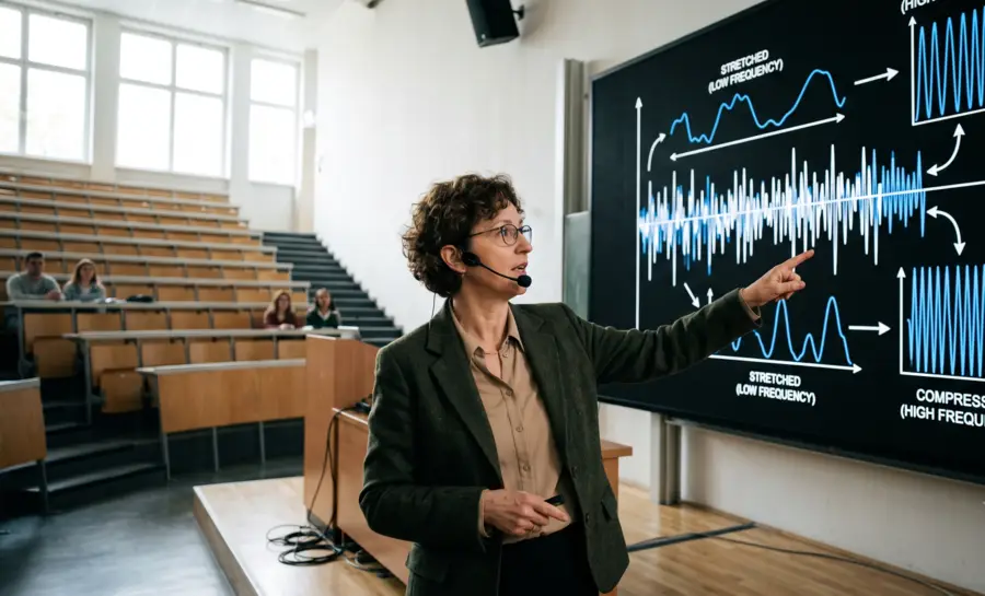
The factor 1/√a normalizes the energy across scales. When a is small, the wavelet is compressed and picks up brief, rapid changes. When a is large, the wavelet is stretched and it captures slow, broad undulations. Translation b moves the wavelet across the time axis, so the analysis slides from start to finish.
The output is a two-dimensional function of time and scale that can be displayed as a scalogram. Back in 1988 researchers such as Ingrid Daubechies formalized the bedrock idea of multiresolution analysis for discrete wavelets, proving that orthonormal bases of compactly supported wavelets can be built with high regularity. The CWT inherits that fundamental scaling and shifting principle, but without the requirement of an orthogonal basis: you can use any mother wavelet that meets a simple admissibility condition, which makes the transform invertible.
This construction gives wavelets their signature strength. Because a mother wavelet is a brief, wave-like pulse it naturally zeroes in on transient events. Scaling and shifting alone deliver a simultaneous view of time and scale, something a fixed-window Fourier approach cannot match without forcing an artificial trade-off between time and frequency resolution.
What Is Discrete Wavelet Transform?
The discrete wavelet transform, or DWT, samples the scale and translation parameters on a structured grid rather than evaluating every possible value. In common constructions, scales and positions change dyadically, often by powers of two. This produces a compact set of coefficients while retaining information at several resolutions.
The DWT is commonly implemented with paired low-pass and high-pass filters. The low-pass branch retains a smoothed approximation of the signal, while the high-pass branch captures detail. Downsampling then reduces the number of samples at each level, and the approximation branch can be decomposed again.
This filter-bank structure makes the DWT efficient for finite digital data. It also supports reconstruction when the analysis and synthesis filters are properly designed.
Applications include denoising, compression, event detection, and multiscale feature extraction, although the interpretation of coefficients remains dependent on sampling, boundary treatment, and wavelet choice.
Discrete Wavelet Transform Explained
The DWT represents a sampled signal through approximation coefficients and detail coefficients at successive levels. At the first level, the signal is separated into broad, slowly varying content and more rapidly changing detail. Repeating the operation on the approximation creates a hierarchy of resolutions.
Unlike the CWT, the DWT does not normally produce coefficients for every continuous position and scale. Its structured sampling reduces redundancy and computational cost. This makes it practical for large arrays, real-time processing, and compression systems.
The decomposition level determines how far the analysis proceeds. Too few levels may miss broad structure, while too many can produce coefficients that are difficult to interpret or strongly affected by the signal length and boundary conditions. The useful depth is therefore a property of the data and the analytical purpose, not a universal constant.
DWT Discrete Wavelet Transform Algorithm Steps
A standard DWT proceeds through repeated filtering and downsampling. The core operation is simple, but each step affects the representation that follows.
Select a wavelet family and the desired decomposition level.
Pass the signal through a low-pass filter to obtain approximation samples.
Pass the same signal through a high-pass filter to obtain detailed samples.
Downsample both outputs and repeat the process on the approximation branch.
Store the coefficients and reconstruct the signal when needed.
The resulting coefficient tree separates coarse structure from progressively finer detail. In practice, reconstruction may be used to test whether selected coefficients preserve the signal features relevant to the analysis.
Haar Wavelet Transform: The Simplest Wavelet
The Haar wavelet is the simplest used wavelet. It is piecewise constant as it takes one value over part of a short interval and the opposite value over another part, with zero average. Its abrupt shape makes it naturally responsive to jumps and step-like transitions.
For a short pair of samples, the Haar transform can be understood as calculating an average and a difference. The average becomes a coarse approximation, while the difference records local change. Repeating this operation creates a multilevel representation with a particularly clear interpretation.
The Haar wavelet is computationally inexpensive and easy to explain, but it is not smooth. Signals dominated by gradual oscillations may be represented less efficiently than they would be with smoother wavelets. Its value is greatest when simplicity, fast calculation, or sensitivity to discontinuities matters more than smooth frequency selectivity.
Choosing a Mother Wavelet
Not every little wiggle qualifies as a mother wavelet. The function must satisfy the admissibility condition, which essentially means it has zero mean and finite energy, meaning it wiggles above and below zero and decays to nothing outside a short interval.
Beyond that requirement, you are free to choose a shape that matches the kind of features you expect in your data. The choice isn’t formulaic, but practical experience points to a few heuristics:
Shape similarity. If your signal contains oscillatory bursts, a Morlet wavelet—a complex sine wave wrapped in a Gaussian—often works well because it resembles a localized oscillation. For sharp, spiky transients, something like the Mexican hat wavelet (the second derivative of a Gaussian) or a compactly supported wavelet can isolate edges and peaks more cleanly.
Time–scale resolution balance. A longer wavelet gives finer discrimination between nearby scales but blurs the exact moment a feature occurs. A shorter wavelet pinpoints timing but mixes scales together. This is the inevitable trade-off of localized analysis, not a flaw.
Real vs. complex wavelets. A real-valued mother wavelet (e.g., the Mexican hat) delivers only amplitude information. A complex wavelet (e.g., the Morlet) yields both amplitude and phase, which can be essential when you later want to examine timing relationships between two signals through cross‑wavelet coherence.
The orthonormal bases of compactly supported wavelets built in Daubechies’ study are meant for discrete, perfect reconstruction tasks. For the CWT, you aren’t tied to orthonormality, so you can freely select non‑orthogonal wavelets if they better match your signal’s morphology.
Still, compact support and regularity remain desirable since they can reduce edge smearing and give clean transforms.
Computing the Continuous Wavelet Transform
In practice, the CWT is approximated by convolving the signal with scaled, time-reversed copies of the mother wavelet. Because signals are finite, the wavelet inevitably extends beyond the edges of the data as it approaches the beginning or end of the record. Those boundary regions produce distorted values; the cone of influence (COI) marks the time‑scale region where edge effects render the analysis unreliable. Any feature that pokes into the COI must be treated with suspicion.
To build a scalogram, scales are typically sampled as fractional powers of two to cover a range that matches the signal’s duration. Computing the squared magnitude of the CWT coefficients yields wavelet power, which is then plotted as a color map with time on one axis, scale on the other.
Interpreting Scalograms
A scalogram is the primary visual output of wavelet analysis. Bright regions correspond to high wavelet power, these are places where the signal has a strong component at a particular scale and time.
But not every hot spot is meaningful. To distinguish genuine features from random fluctuations, researchers often derive statistical significance tests against theoretical backgrounds: white noise (which spreads power evenly) and red noise (which concentrates power at low frequencies, as many natural processes do). By comparing observed power to the 95th percentile of the background spectrum, you can identify epochs and scales that are unlikely to have arisen by chance.
Smoothing in time, in scale, or both can increase the reliability of such features.
Known Limitations and Cautions of CWT
No mathematical tool is without its soft spots, and the CWT is no exception. Mother wavelet choice is both a flexibility and a liability. There is no automatic procedure that guarantees the optimal wavelet for an unknown signal.
An inappropriate choice—say, a long Morlet for a signal full of sharp spikes—can smear features or create misleading scalogram artifacts. Even when experimenters land on a good match by eye, the analysis remains partly subjective.
Edge effects are a physical reality of finite data. Long scales push the wavelet far beyond the boundaries, so the COI can swallow a large portion of the scalogram at the coarsest scales. Any event inferred from the margins must be treated as tentative. Significance tests, while principled, hinge on assumed noise models that may not hold for every dataset.
When approaching a new dataset, the clearest path combines physical reasoning about the signal’s expected structure with conservative statistical checks, and a clear-headed acceptance that the scalogram is a suggestive map, not a definitive anatomical blueprint.
Using Wavelet Transform for EEG Analysis
Electroencephalography records voltage changes over time, and those changes often contain overlapping rhythms, transient events, and non-stationary behavior. A wavelet transform can represent these components across time and scale, making it useful for examining when particular patterns emerge. The method is therefore relevant to neuroscience and to the analysis of EEG recordings.
In EEG work, coefficients may be summarized by scale, time interval, channel, or event condition. Such summaries can support research into rhythms, evoked responses, seizure-related transients, sleep patterns, or artifact structure. The transform itself does not diagnose a brain disorder; interpretation requires appropriate acquisition, preprocessing, comparison groups, and domain expertise.
Preprocessing remains central. Electrode artifacts, eye movements, muscle activity, reference choices, filtering, missing data, and edge effects can all alter wavelet coefficients. Results are also sensitive to the frequency-to-scale mapping and to whether the selected wavelet resembles the temporal morphology being studied.
Tools and Software for Computing Wavelet Transforms
Wavelet transforms can be computed with numerical libraries, scientific programming environments, and specialized signal-processing software. The appropriate choice depends on whether the goal is teaching, exploratory visualization, batch processing, embedded computation, or reproducible research.
A useful tool should expose the transform parameters clearly rather than hiding them behind a single default command.
A typical workflow loads and validates the sampled data, chooses a wavelet, computes the CWT or DWT, inspects coefficients, and evaluates reconstruction or downstream features. Repeating the workflow with controlled parameter changes can show whether the result is stable. Documentation and version records matter when small implementation differences affect coefficient values.
For reliable work, software evaluation often includes numerical accuracy, support for multidimensional data, boundary options, plotting, computational cost, and interoperability. Code should also preserve the sampling rate and preprocessing history, since coefficients without that context are difficult to reproduce or interpret.
Why Wavelet Analysis Matters for Reading Non-Stationary Signals
The wavelet transform's defining insight is that a signal's identity is best understood not as a static list of frequencies but as a living map of when patterns occur and how long they last. This time-scale view has proven its worth in real-world settings. Yet those successes always carry a caveat: the analysis is only as trustworthy as the choices made before the math begins.
Choosing a mother wavelet is a matter of scientific judgment, and edge effects plus noise assumptions place real boundaries on what any scalogram can claim. The honest takeaway is that wavelet analysis offers a way to see structure in changing signals, but it demands conservative interpretation rather than blind acceptance of every bright spot.
Researchers who pair physical reasoning with statistical checks get the most value from this tool while keeping their conclusions appropriately modest.
References
Daubechies, I. (1988). Orthonormal bases of compactly supported wavelets. Communications on pure and applied mathematics, 41(7), 909-996. https://doi.org/10.1002/cpa.3160410705
Torrence, C., & Compo, G. P. (1998). A practical guide to wavelet analysis. Bulletin of the American Meteorological society, 79(1), 61-78. https://doi.org/10.1175/1520-0477(1998)079%3C0061:APGTWA%3E2.0.CO;2
Frequently Asked Questions
What is the wavelet transform and why is it used for non-stationary signals?
The wavelet transform decomposes a signal into components that are localized in both time and scale, revealing when a pattern appears and at what duration it operates. It is built for non-stationary signals, whose character changes over time, unlike fixed approaches that assume steady behavior.
How does the continuous wavelet transform differ from Fourier analysis?
Instead of breaking a signal into endless sine waves, the CWT uses scaled and translated copies of a single mother wavelet. This construction provides a simultaneous view of time and scale, avoiding the fixed-window trade-off between time and frequency resolution found in Fourier methods.
What is a mother wavelet and what condition must it satisfy?
A mother wavelet is a single, localized oscillating function that is stretched and shifted to analyze a signal. To be valid, it must satisfy the admissibility condition, which essentially means it has zero mean and finite energy—it wiggles above and below zero and decays to nothing outside a short interval.
How do you choose a mother wavelet for a particular signal?
Choose a wavelet whose shape matches the features you expect; for example, a Morlet wavelet suits oscillatory bursts, while a Mexican hat wavelet isolates sharp spikes. You also balance time versus scale resolution and decide whether you need phase information, with complex wavelets offering both amplitude and phase.
What is a scalogram and how do you interpret it?
A scalogram is the main visual output of wavelet analysis, plotting wavelet power with time on one axis and scale on the other. Bright regions indicate strong signal components at a particular time and scale, but significance tests against white or red noise backgrounds help distinguish genuine features from random fluctuations.
What is the cone of influence and why does it matter?
The cone of influence marks the time-scale region where edge effects make wavelet analysis unreliable because the wavelet extends beyond the finite data boundaries. Any feature that falls inside the COI must be treated with suspicion.
What are the main limitations of the continuous wavelet transform?
The choice of mother wavelet is partly subjective, and an inappropriate choice can smear features or create misleading artifacts. Edge effects can contaminate large areas of the scalogram, and significance tests rely on assumed noise models that may not hold for every dataset.
How do real and complex mother wavelets differ in practice?
Real-valued wavelets, such as the Mexican hat, provide only amplitude information. Complex wavelets, such as the Morlet, provide both amplitude and phase, which is essential for examining timing relationships between signals through cross-wavelet coherence.
What is the difference between CWT and DWT?
The continuous wavelet transform evaluates many closely spaced scales and positions, producing a detailed and often redundant representation. The discrete wavelet transform uses a structured set of scales and positions to produce a more compact representation.
What is the Haar wavelet used for?
The Haar wavelet is useful for simple, fast analysis of signals with abrupt changes or step-like behavior. Its piecewise-constant form also makes the underlying averages and differences easy to interpret.
Emotiv is a neurotechnology leader helping advance neuroscience research through accessible EEG and brain data tools.
Medical Disclaimer: The information provided on this website is for educational and informational purposes only and is not intended as medical or health advice. This content may contain errors and should not be relied upon to make life-altering health, medical, or lifestyle choices. Always seek the advice of your physician or other qualified health provider with any questions you may have regarding a medical condition or treatment.
Christian Burgos