Principal component analysis, usually shortened to PCA, is one of the mathematical tools proposed that offers a way to simplify multichannel EEG recordings, reduce how much data needs to be processed, and flag the loudest, most disruptive artifacts, all without making some of the stricter statistical assumptions that other artifact-removal methods require.
This article explains what PCA actually does to EEG data, how researchers have used it in real preprocessing pipelines, and what the current, still-limited evidence says about whether it works as advertised.
What Is Principal Component Analysis in EEG?
To understand further PCA, it helps to picture what raw EEG data looks like before any signal processing happens.
A typical recording involves many electrodes, each producing its own continuous stream of voltage readings over time. These channels are not independent of each other. Because they are all picking up electrical activity from a shared, conductive medium (the head), their signals overlap and correlate in complicated ways.
PCA takes this tangle of correlated channels and reorganizes it into a new set of signals called components. Each component is a weighted combination of the original channels, but with one critical mathematical property: the components are orthogonal, meaning they are uncorrelated with each other.
PCA also ranks these components by how much variance, or overall signal variation, each one accounts for. The first component captures the largest share of variance in the data, the second captures the next largest share among what remains, and so on down the list.
This ranking is crucial because of how artifacts tend to behave. Eye blinks, for example, produce large, slow voltage swings that spread widely across many electrodes at once. Because this creates a big, shared pattern of variation, blink activity tends to concentrate in the highest-variance components. Weaker, more localized brain signals often end up further down the list, in lower-variance components.
One detail separating PCA from some of its better-known cousins like independent component analysis (ICA) is that it does not assume the underlying sources are statistically independent. It only requires that the resulting components be uncorrelated, which is a much looser condition.
How Does Principal Component Analysis (PCA) Work? A Step-by-Step Explanation
Step 1: Standardize the Data
Before launching a complex calculation, one must normalize the input to ensure parity across variables. If one variable is measured in microvolts and another in milliseconds, the raw differences in scale would bias the results. Scaling each variable to a mean of zero and a standard deviation of one allows the math to treat all input features with equal weighting.
Step 2: Calculate the Covariance Matrix
Once the data is standardized, the next hurdle is mapping out the relationships between every pair of features. A covariance matrix summarizes these interactions, showing which variables move together and which are independent. This grid serves as the foundation for identifying the directions where the dataset exhibits the most significant spread.
Step 3: Compute Eigenvectors and Eigenvalues
This stage involves solving for the specific vectors that characterize the shape of the data distribution. Eigenvectors determine the direction of the new axes, while eigenvalues represent the magnitude of variance captured along those specific directions. These mathematical markers allow us to rotate the original data space into a new coordinate system defined by the primary patterns of movement.
Step 4: Select Principal Components
After identifying the components, the analysis restricts the model to only those that explain a significant portion of the total variance. This filtering process discards noise-heavy variables and retains only the most informative patterns according to specific quantitative thresholds.
By focusing strictly on dominant components, researchers reduce the computational burden on subsequent processing tasks. This ensures that the final model is both responsive and efficient for real-time analysis.
Step 5: Transform the Original Data
With the final selection complete, the last step is projecting the original observation points onto these new axes. This transformation creates a new, reduced-dimension dataset that preserves the essential topography of the original measurements.
Professionals then use these transformed variables for downstream tasks like classification or source localization, benefiting from a cleaner signal representation.
How PCA Fits Into the EEG Preprocessing Pipeline
In practice, PCA rarely works alone. It tends to show up as a step inside a larger cleaning pipeline, performing one of two jobs:
Shrinking the data down
Helping detect where the artifacts are hiding
The first role is dimensionality reduction. A study combining PCA with a technique called density estimation blind source separation, or DEBSS, used PCA specifically to reduce the size of the EEG dataset before further separation could occur.
In this pipeline, high-frequency noise was first filtered out using wavelet analysis, and then “the PCA algorithm is used to process the EEG signals to reduce the data dimension” before DEBSS took over to separate the remaining components. Once the interference-carrying components were identified using cross-correlation coefficients and related nonlinear parameters, the researchers reconstructed the signal from the remaining, cleaner components.
The second role is artifact detection itself, and it appears inside a widely used method called Artifact Subspace Reconstruction, or ASR. ASR works by continuously analyzing short windows of EEG data and comparing them against a baseline of “clean” activity.
According to a 2019 study introducing a Riemannian version of this method, ASR “repeatedly computes a PCA on covariance matrices to detect artifacts based on their statistical properties in the component subspace”. Here, PCA is not reducing the number of channels for convenience. It is functioning as the engine that decides, moment to moment, whether a segment of data looks statistically normal or looks like an artifact.
Taken together, these two examples conclude that PCA is a component of a cleaning strategy, not a complete cleaning strategy by itself. It typically hands off its output to another algorithm, whether that is DEBSS, a Riemannian geometry adaptation, or another decision-making process that determines which components actually get removed.
Can PCA Isolate EEG Artifacts? What the Evidence Shows
The reasoning behind PCA's appeal for artifact isolation is straightforward. Because PCA sorts components by variance, and because blinks and muscle activity tend to generate outsized voltage swings, the neuroscience theory holds that these artifacts should naturally sort themselves into the top few components. If that holds true, a researcher could, in principle, isolate and discard the worst interference quickly, without needing to model the exact statistical independence of every brain source.
The study that tested the PCA-plus-DEBSS pipeline described earlier reported that the combined method “can eliminate the main interference of multi-channel EEG signals rapidly and effectively,” while also noting that the approach was “stable and has strong scalability.” This is a positive result, but it is worth noting precisely what was tested: a specific two-step pipeline, not PCA operating in isolation.
The aforementioned 2019 study took a more structured comparative approach. The researchers built a Riemannian-geometry-based version of ASR, called rASR, and tested it against the standard PCA-based ASR method using EEG recorded on smartphones in both indoor and outdoor conditions, with 27 participants.
They evaluated performance across three separate measures:
How well each method reduced eye-blink artifacts (sensitivity)
How well each method preserved visual-evoked potentials, which are brain responses to visual stimuli (specificity)
How quickly each method ran (efficiency)
According to the author’s conclusions, rASR “performed favorably on all three measures” when compared to standard ASR.
These results are encouraging for PCA-based artifact handling, but the evidence base behind them is narrow. These are meaningful, useful early findings, but they do not yet amount to a broadly validated claim that PCA reliably isolates artifacts across all EEG contexts.
PCA vs. ICA vs. Filtering: Choosing the Right Tool
EEG researchers have several tools available for cleaning data, and PCA occupies a specific niche among them.
Filtering, which includes high-pass, low-pass, and notch filters, works by removing or dampening entire frequency bands. This is useful for removing steady interference like electrical line noise, but it runs into a hard limit when an artifact and a brain signal share the same frequency range.
A blink, for instance, can overlap in frequency with slow brain waves, and a filter cannot tell them apart because it only sees frequency, not the pattern of variance across channels. PCA operates on a completely different axis as it looks at how signal variation is distributed across the whole set of electrodes, not at frequency content. This makes it a complementary approach rather than a direct substitute for filtering.
On the other hand, ICA is often mentioned in the same breath as PCA, but the two methods rest on different assumptions. ICA searches for components that are statistically independent from one another, a much stronger and more computationally demanding requirement than PCA's looser condition of simple decorrelation.
Because ICA has to search harder for this stricter kind of separation, it tends to require more computing time and more data. PCA, being mathematically simpler, is faster and does not need independence at all, only that the resulting components be uncorrelated.
This difference in computational cost is why PCA frequently shows up as a preparatory step before ICA rather than as its replacement. Reducing the number of dimensions with PCA first can speed up an ICA run and reduce the risk of overfitting when data is limited. Alternatively, PCA can act as a coarse first pass, removing the most dominant, obvious artifacts before a more careful method fine-tunes the rest.
Method | Separation Basis | Speed | Key Limitation |
|---|---|---|---|
PCA | Sorts by variance | Fast | Variance ≠ artifact |
ICA | Finds independent sources | Slow | Assumes independence |
Filtering | Removes frequency bands | Very fast | Overlapping frequencies remain |
Limitations of PCA-Based Artifact Removal
PCA's simplicity is also the source of its weaknesses. Several open questions remain about how well it actually performs the artifact-isolation job it is often assigned.
Variance is an imperfect stand-in for “artifact.” Certain brain rhythms, such as posterior alpha activity (a well-known EEG rhythm associated with relaxed, eyes-closed states), can produce high-amplitude signals in their own right. A method that assumes high variance always means artifact risks discarding genuine brain activity along with the noise it is meant to remove.
In the other direction, blink artifacts do not always confine themselves neatly to a single component; their influence can spread across several components at once, complicating any simple “remove the top component” strategy.
There is also a structural mismatch to consider. PCA forces its components to be orthogonal to one another by mathematical definition. But there is no guarantee that the actual physical sources generating EEG signals, whether they are neural circuits or muscle groups near the scalp, are arranged in a way that matches this orthogonal geometry.
When the assumption does not match the underlying reality, the separation PCA produces may be a mathematical convenience rather than an accurate reflection of what is actually happening in the tissue.
Practical Advice for Using PCA in EEG Analysis
For someone exploring an EEG dataset for the first time, PCA remains a reasonable starting point, particularly as a way to see which patterns of variation dominate a given recording. Here are some tips that are often recommended:
Use PCA as a preliminary step to reduce dimensionality or flag dominant artifact patterns, not as a final cleaning pass.
Combine PCA with a subsequent method (e.g., ICA, DEBSS, ASR) that can decide which components to remove.
Always visually inspect the scalp topography and time course of discarded components to verify they represent artifacts.
Treat variability in results across recording environments (lab vs. mobile) with caution and validate on your own data.
Conclusion: Is PCA a Reliable EEG Cleaning Method?
PCA transforms messy brainwave data into ranked components, giving researchers a quick way to zero in on the noisiest parts of a recording. This approach is especially useful when eye blinks or muscle movements dominate the signal, as they often bubble up to the highest-variance slots.
But because genuine brain rhythms can also produce strong signals, the method cannot be trusted on its own to decide what is an artifact and what is precious neural data.
References
Kang, D., & Zhizeng, L. (2012, March). A method of denoising multi-channel EEG signals fast based on PCA and DEBSS algorithm. In 2012 International Conference on Computer Science and Electronics Engineering (Vol. 3, pp. 322-326). IEEE. https://doi.org/10.1109/ICCSEE.2012.105
Blum, S., Jacobsen, N. S. J., Bleichner, M. G., & Debener, S. (2019). A Riemannian Modification of Artifact Subspace Reconstruction for EEG Artifact Handling. Frontiers in human neuroscience, 13, 141. https://doi.org/10.3389/fnhum.2019.00141
Frequently Asked Questions
What is principal component analysis (PCA) in the context of EEG?
PCA is a mathematical method that reorganizes multichannel EEG data into a new set of signals called components, which are uncorrelated with each other. It ranks these components by how much variance they capture, with the first component explaining the most overall signal variation.
How does PCA help with removing artifacts from EEG data?
Because artifacts like eye blinks produce large, widespread voltage swings, they tend to concentrate in the highest-variance components. PCA’s ranking by variance allows researchers to identify and potentially discard those top components, which often contain the most disruptive noise.
Does PCA work alone to clean EEG signals?
No, PCA is rarely used as a standalone cleaning solution. It typically acts as a step within a larger pipeline, either reducing data dimensions before applying another method like DEBSS, or serving as the detection engine inside a framework like Artifact Subspace Reconstruction (ASR).
What is the difference between PCA and ICA for artifact removal?
PCA only requires the resulting components to be uncorrelated, which is a looser mathematical condition, while ICA searches for components that are statistically independent, a stricter and more computationally demanding requirement. PCA is faster and often used as a preparatory step before ICA rather than a replacement for it.
Can PCA accidentally remove real brain activity along with artifacts?
Yes, because PCA relies on variance to identify artifacts, high-amplitude brain rhythms like posterior alpha activity can be mistaken for noise. Additionally, artifacts may spread across multiple components, so simply removing the top component can discard genuine neural signals.
How does PCA compare to frequency filtering for EEG cleaning?
Frequency filtering removes or dampens signal energy in specific frequency bands, but it cannot separate an artifact and a brain signal that share the same frequencies. PCA looks at patterns of variance across all electrodes instead, making it a complementary approach that addresses a different dimension of the data.
How should a researcher use PCA safely in an EEG preprocessing workflow?
PCA can be used as a dimensionality reduction step before applying other methods, or as a helper to inspect which patterns dominate a recording. Researchers should visually inspect the components they plan to discard by checking their scalp topography and time course, rather than blindly trusting the variance ranking.
Emotiv is a neurotechnology leader helping advance neuroscience research through accessible EEG and brain data tools.
Medical Disclaimer: The information provided on this website is for educational and informational purposes only and is not intended as medical or health advice. This content may contain errors and should not be relied upon to make life-altering health, medical, or lifestyle choices. Always seek the advice of your physician or other qualified health provider with any questions you may have regarding a medical condition or treatment.
Christian Burgos