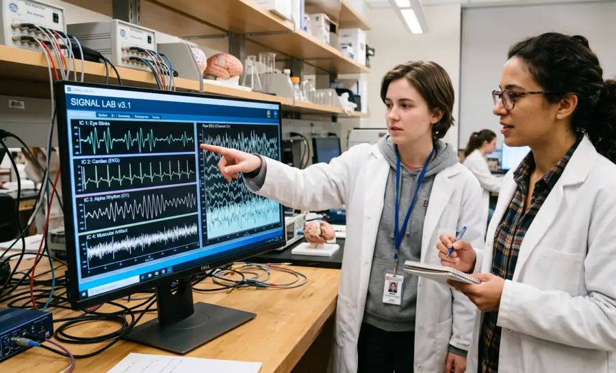
Independent component analysis is a powerful computational method for blind source separation used across diverse fields. It effectively disentangles mixed EEG signals that are statistically independent and non-Gaussian.
What is Independent Component Analysis (ICA)?
Independent component analysis is a sophisticated statistical and computational technique focused on extracting hidden factors or components from a set of mixed observations.
In many real-world scenarios, recorded data is the result of multiple source signals acting simultaneously through a medium, creating a complex overlap that is often unintelligible in its raw form. By implementing specific algebraic transformations, this method acts as a filter to reverse the mixing process.
The Core Concept: Separating Mixed Signals
The fundamental premise of the field revolves around the "cocktail party problem," where multiple people speak at once in a room while several microphones record the resulting auditory mess.
A casual observer hears only a chaotic blend of voices, but ICA can theoretically identify the signal contributed by each individual speaker. This capability allows researchers to isolate specific waveforms from a global stream, providing a clear window into individual data channels that would otherwise be obscured.
Mathematical Foundations of ICA
Mathematically, the goal is to perform a blind source separation, finding a linear transformation that renders the observed variables as independent as possible. Given an observed vector of data, the algorithm seeks an unmixing matrix that, when multiplied by the observations, yields estimated source signals that have independent statistical distributions.
Achieving this requires that these signals be non-Gaussian, as the mathematical properties of Gaussian distributions make them impossible to separate uniquely. In the context of modern neuroscience, this rigor ensures that subtle electrical fluctuations are not lost to the background noise of surrounding interference.
How Does Independent Component Analysis Work?
Operating successfully with high-dimensional data, the process relies on transforming a mixture into its constituent parts by measuring non-Gaussianity. Because mixed signals often tend toward a Gaussian distribution due to the central limit theorem, the algorithm functions by aggressively searching for directions in the data that are as far from Gaussian as possible.
The resulting components are effectively "pure" signals that reconstruct the original source independent of the mixing process.
Assumptions of ICA
Successful execution of this algorithm rests upon several critical requirements. The most important assumption is that the source signals are statistically independent from one another; if knowing the value of one source provides no information about another, they qualify for separation.
Additionally, the algorithm assumes the number of observed mixed signals is at least as large as the number of independent sources. Finally, as noted, the sources must exhibit non-Gaussian distributions, as this distinct structure creates the landmarks the algorithm needs to anchor its separation efforts.
Independent Component Analysis Algorithm: Key Techniques
Several algorithmic approaches exist to achieve this separation, with FastICA and Infomax being among the most prominent examples. These methods iteratively adjust the unmixing matrix to minimize the mutual information or maximize the non-Gaussianity of the outputs.
The optimization process is computationally intensive, requiring careful implementation to ensure consistent convergence across different datasets. By refining these weights, the system progressively peels back the layers of interference until each distinct signal emerges clearly.
Independent Component Analysis vs. Principal Component Analysis (ICA vs. PCA)
While both techniques are used for dimension reduction or signal analysis, their functional goals diverge significantly. Researchers must choose between them based on whether they seek to capture variance or independence within their dataset.
Feature | Principal Component Analysis | Independent Component Analysis |
|---|---|---|
Primary Focus | Maximum Variance | Maximum Independence |
Orthogonality | Required | Not Required |
Component Order | Sorted by Eigenvalues | Randomly Ordered |
Statistical Measure | Correlations | Higher-order Statistics |
Selecting the correct tool depends on the specific goals of the underlying analysis. While PCA is excellent for data compression where preserving the main trends is key, ICA is superior when the goal is identifying unique, independent processes contributing to the total observation.
How Independent Component Analysis Separates Brain Signals from Noise
Independent Component Analysis takes a stricter approach than PCA. Instead of just decorrelating signals, ICA searches for components that are statistically independent, meaning knowing the value of one component provides no information whatsoever about any other component.
This is a much higher bar than decorrelation, and it is what allows ICA to pull apart signals that share frequency content but originate from genuinely separate physical sources: a blink here, a jaw clench there, a patch of visual cortex responding to a stimulus somewhere else.
Winkler et al. study applies TDSEP, a version of ICA that factors in temporal correlations across time, not just the instantaneous statistics of the signal.
Olaf Dimigen study uses Infomax, a widely used ICA algorithm.
Mognon study builds its automated detection tool on top of a general ICA-based pipeline.
Despite differences in implementation, all of these approaches rest on the same underlying principle: decompose the mixed electrode signal into a set of components that behave independently of one another, then figure out which of those components look like brain activity and which look like an artifact.
The Core Assumptions Behind ICA: Non-Gaussianity and Linear Mixing
ICA works because of two specific assumptions about the data, and understanding them explains both its strengths and its failure points.
The first assumption is non-Gaussianity. True EEG sources, whether they are brain rhythms, eye blinks, or muscle bursts, tend to have amplitude distributions that deviate from the bell-curve shape of a Gaussian (normal) distribution. ICA algorithms are built to seek out and maximize this non-Gaussian structure, because a mixture of independent signals tends to look more Gaussian than any of its individual components (a consequence of the central limit theorem).
The second assumption is linear mixing. ICA assumes that what an electrode records is an instantaneous, linear combination of underlying source signals, an assumption that holds reasonably well for how electrical activity spreads through tissue and skull (a process known as volume conduction) in stable recording conditions. This assumption is easiest to satisfy when a person sits still.
Why High-Pass Filtering Before ICA Changes Everything
The quality of an ICA decomposition depends heavily on how the signal is processed before the algorithm ever runs, and the choice of high-pass filter cutoff (a filter that removes very slow drifts below a set frequency) turns out to be one of the most consequential decisions in the entire pipeline.
A 2015 study led by Winkler et al. tested this directly using event-related potential (ERP) data, brainwave patterns time-locked to a specific stimulus, from 21 participants performing an auditory oddball task. High-pass filtering between 1 and 2 Hz consistently produced good results across three separate metrics: signal-to-noise ratio, single-trial classification accuracy, and the percentage of components that looked “near-dipolar,” meaning they had a spatial pattern consistent with a single, localized brain source rather than a smeared mix of several sources.
Moreover, in a 2020 study, Klug et al. examined the same question across stationary and mobile recording setups. For a standard stationary experiment with 64 channels and a 0.5 Hz filter, results were acceptable. But mobile experiments required a higher cutoff, up to 2 Hz, to reach an optimal decomposition, and setups with more channels needed correspondingly higher filters.
Olaf Dimigen research pushed this idea further in the specific context of eye movement artifacts. Systematically varying the high-pass filter, low-pass filter, and the proportion of training data containing saccadic spike potentials, the researcher found that training the ICA on data where these spike potentials were massively overweighted strongly improved correction quality.
Together, these three studies point to the same conclusion: default filter settings, particularly the common 0.5 Hz cutoff, may be too permissive for many use cases, and the correct choice depends on the specific artifact and recording conditions.
Automating Artifact Component Selection with Machine Learning
Once ICA produces a set of independent components, someone or something still has to decide which components represent brain activity and which represent artifacts. Manual labeling by trained experts is slow and introduces subjectivity, since different experts do not always agree on borderline cases.
To address this, Winkler’s team built a subject-independent linear classifier using just six features drawn from frequency, spatial, and temporal characteristics of each component. Trained on 640 hand-labeled TDSEP components from 12 participants in a reaction-time study, the classifier achieved less than 10% Mean Squared Error (MSE) when tested on new data, a performance level on par with the natural disagreement rate between human experts.
When applied without retraining to a completely different auditory ERP paradigm, the same classifier reached 15% MSE, a reasonable but noticeably weaker result that reflects the difficulty of generalizing across paradigms. In a motor imagery brain-computer interface task, the researchers demonstrated that removing up to 60% of the most artifactual components still preserved the discriminant information needed for the BCI to function.
Furthermore, Mognon’s team introduced ADJUST, a fully automatic algorithm that combines spatial and temporal features specifically tuned to detect blinks, eye movements, and generic discontinuities. Validated on an independent dataset, ADJUST's classification of components agreed with manual expert labeling on 95.2% of the data variance. Removing the components ADJUST flagged as artifactual produced what the study describes as neat reconstruction of visual and auditory event-related potentials from heavily artifacted data.
Both tools represent real progress toward reducing the manual burden of EEG cleaning, but their reported performance comes from specific datasets and paradigms, and generalization to new conditions is not guaranteed.
Practical Takeaways for Cleaning EEG Data with ICA
Independent Component Analysis works because it targets true statistical independence rather than the weaker property of decorrelation that methods like PCA rely on. This distinction is what allows it to pull apart brain signals and artifacts even when their frequency content overlaps, something frequency-domain filtering cannot do and something regression-based EOG correction failed to achieve in direct testing.
That success, however, is conditional. High-pass filtering in the 1 to 2 Hz range has been shown to produce consistently good decompositions in stationary ERP research, while mobile recordings benefited from filters up to 2 Hz, with channel count also playing a role. For especially difficult artifacts like saccadic spike potentials during free viewing, deliberately overweighting the artifact during training, rather than using default settings, can turn an unsatisfactory correction into one that removes nearly all contamination with minimal distortion of brain activity.
Further, automated component classifiers, including the six-feature linear model from the and the ADJUST algorithm from the aforementioned studies, can meaningfully cut down the time and subjectivity involved in manual labeling. Both showed strong agreement with expert judgment on their validation data. However, neither should be treated as a universal solution without some awareness of how performance can shift across different recording paradigms and equipment.
ICA-based artifact removal remains one of the more well-supported approaches available for cleaning EEG data, and the neuroscience behind it is grounded in a coherent statistical logic. But its actual performance depends on choices made long before the algorithm runs: filter settings, training data composition, and the specific artifact being targeted. Anyone applying it should validate results with objective metrics rather than assuming a single configuration will work everywhere.
Why Preprocessing Choices Define the Success of ICA in EEG
Clean brain data is the foundation for everything from thought-controlled devices to careful memory research. Independent Component Analysis provides a mathematically sound way to pull apart mixed neural activity and bodily noise, even when simpler methods like simple filtering fall short. By targeting true statistical independence, it can reveal the separate electrical fingerprints of a real brain rhythm and an eye blink that occur in the same frequency band.
The real power, however, emerges only when researchers move beyond plug-and-play defaults. The studies show that tuning the high-pass filter to the specific recording situation and carefully preparing the training examples for artifact detectors are what turn ICA from a hopeful experiment into a consistently reliable tool. Paying this kind of personalized attention allows scientists to confidently recover the brain’s messages instead of leaving them scrambled inside a noisy recording.
References
Winkler, I., Haufe, S., & Tangermann, M. (2011). Automatic classification of artifactual ICA-components for artifact removal in EEG signals. Behavioral and brain functions, 7(1), 30. https://doi.org/10.1186/1744-9081-7-30
Dimigen, O. (2020). Optimizing the ICA-based removal of ocular EEG artifacts from free viewing experiments. NeuroImage, 207, 116117. https://doi.org/10.1016/j.neuroimage.2019.116117
Mognon, A., Jovicich, J., Bruzzone, L., & Buiatti, M. (2011). ADJUST: An automatic EEG artifact detector based on the joint use of spatial and temporal features. Psychophysiology, 48(2), 229-240. https://doi.org/10.1111/j.1469-8986.2010.01061.x
Winkler, I., Debener, S., Müller, K. R., & Tangermann, M. (2015). On the influence of high-pass filtering on ICA-based artifact reduction in EEG-ERP. Annual International Conference of the IEEE Engineering in Medicine and Biology Society. IEEE Engineering in Medicine and Biology Society. Annual International Conference, 2015, 4101–4105. https://doi.org/10.1109/EMBC.2015.7319296
Klug, M., & Gramann, K. (2021). Identifying key factors for improving ICA‐based decomposition of EEG data in mobile and stationary experiments. European Journal of Neuroscience, 54(12), 8406-8420. https://doi.org/10.1111/ejn.14992
Frequently Asked Questions
Why can't simple frequency filtering remove EEG artifacts like eye blinks and muscle activity?
Frequency filtering fails because artifacts and brain signals often share the same frequency bands, such as muscle activity and frontal theta rhythms, so removing one also removes the other. A filter cannot separate them when their oscillations overlap.
What is the key difference between PCA and ICA in separating brain signals from noise?
PCA only decorrelates signals—it makes them linearly uncorrelated—but does not require statistical independence. ICA goes further by searching for components that are completely statistically independent, meaning knowing one reveals nothing about another, which enables better separation of mixed brain and artifact sources.
How does ICA actually separate brain signals from artifacts?
ICA assumes that the mixed electrode signals are linear combinations of independent, non-Gaussian source signals. It finds a transformation that maximizes the independence of the resulting components, effectively isolating distinct physical sources like an eye blink from a brain rhythm even if their frequencies overlap.
Why is non-Gaussianity important for ICA to work?
Real EEG sources tend to have non-Gaussian amplitude distributions, while mixtures of independent signals become more Gaussian. ICA algorithms seek and maximize this non-Gaussian structure to pull apart the original sources, because finding the least Gaussian projections recovers the independent components.
Why is high-pass filtering of EEG data before ICA so critical?
The high-pass filter removes very slow drifts that can corrupt the ICA decomposition. Studies consistently found that filter cutoffs around 1–2 Hz produced cleaner, more brain-like independent components compared to lower default settings like 0.5 Hz, especially in mobile recordings or when targeting specific artifacts.
How can machine learning help automate the classification of ICA components as brain or artifact?
Automated classifiers use a few features from each component’s frequency, spatial, and temporal patterns to label them with accuracy close to expert agreement. This reduces the manual, subjective workload of picking which components to remove, though performance may drop when applied to new experimental paradigms.
What happens to ICA performance during mobile EEG recordings where participants move around?
Movement does not break the linear mixing assumption entirely, so ICA still works, but it reduces the number of clean, interpretable brain components that can be recovered. Mobile setups often require a higher high-pass filter cutoff to maintain optimal decomposition compared to stationary recordings.
Can ICA be applied to non-linear mixtures?
The standard algorithm assumes a linear mixture, so applying it to complex non-linear combinations often requires specialized modifications or extensions to the model.
Emotiv is a neurotechnology leader helping advance neuroscience research through accessible EEG and brain data tools.
Medical Disclaimer: The information provided on this website is for educational and informational purposes only and is not intended as medical or health advice. This content may contain errors and should not be relied upon to make life-altering health, medical, or lifestyle choices. Always seek the advice of your physician or other qualified health provider with any questions you may have regarding a medical condition or treatment.
Christian Burgos