An electroencephalogram (EEG) generates vast amounts of continuous data across dozens of channels over long periods. This volume strains the limited memory of portable headsets, constrains telemedicine networks, and slows real-time brain-computer interfaces (BCIs). Consequently, raw EEG data requires reduction to be processed efficiently.
The discrete cosine transform (DCT), which serves as the mathematical foundation for JPEG compression, resolves this challenge. Just as it compresses images while maintaining recognizability, the DCT reduces EEG signal size while preserving its overall shape. Recognizing its mechanics and boundaries helps determine when the DCT is suitable or when alternative transforms are preferable.
What Is the Discrete Cosine Transform?
The discrete cosine transform is a mathematical operation that converts a finite sequence of sampled values into coefficients associated with cosine functions. Instead of describing a signal directly as values over time or position, it describes how strongly different cosine patterns contribute to that signal. The result remains finite and discrete, but its structure is expressed in a frequency-like domain.
A cosine basis begins with a constant pattern and progresses through increasingly rapid oscillations. The first coefficient therefore commonly reflects the average or overall level of the input, while later coefficients capture progressively finer changes. This arrangement can make broad trends easier to separate from rapid fluctuations.
The transform is reversible when the full set of coefficients and the corresponding normalization are retained. In practical work, however, analysts may preserve only selected coefficients or use them as numerical features. That choice can reduce dimensionality, but it also discards information, so the meaning of the reduced representation must be assessed rather than assumed.
The Discrete Cosine Transform Algorithm Step by Step
A practical DCT workflow starts with a finite sequence and ends with coefficients that can be reconstructed or analyzed. The sequence may be a short signal window, an image row, or another ordered collection of measurements. Before calculation, the analyst defines the transform type, coefficient scaling, window length, and treatment of missing or contaminated samples.
Each DCT basis function is a sampled cosine pattern. The algorithm compares the input with every basis pattern, producing one coefficient per pattern. The calculation can be performed directly with the summation formula or with a fast implementation designed to reduce computation while preserving the selected transform convention.
A compact workflow is useful when implementing the operation because each step affects interpretation:
Prepare a finite, consistently sampled sequence.
Remove or model unwanted offsets and trends when the analysis requires it.
Select the DCT type and normalization convention.
Compute the coefficient vector and verify its dimensions.
Retain, reconstruct, or statistically analyze coefficients according to the research question.
After transformation, reconstruction with all coefficients should reproduce the input apart from numerical precision and normalization conventions. A reconstruction using only part of the coefficient vector is an approximation. Examining the reconstruction error can show whether coefficient reduction has removed meaningful structure rather than merely reducing noise.
Discrete Cosine Transform Applications Across Industries
The discrete cosine transform has applications wherever finite, sampled data can benefit from a cosine-based representation. In image and video systems, it supports compact descriptions of spatial or temporal blocks. In audio and communications, related transform methods can help organize signal information for coding and transmission.
Scientific and engineering applications use the DCT for filtering, denoising, feature construction, and numerical analysis. Its real-valued basis can be convenient when phase is not the primary quantity of interest or when a finite sequence with even-extension behavior is a suitable model. The appropriate use depends on the signal, the boundary conditions, and the desired output.
In biomedical research, transform coefficients may serve as features for statistical models or classification systems. Such features are measurements of a transformed signal, not direct biological variables. Their value must therefore be established through validation, reproducibility, and comparison with the original data and relevant physiological measures.
Discrete Cosine Transform vs Discrete Fourier Transform
The DCT and DFT both express sampled data through oscillatory basis functions, but they make different mathematical assumptions. The DFT uses complex exponentials and represents both amplitude and phase in its coefficients. The DCT uses real cosine functions and is commonly associated with an even-symmetric extension of the finite input.
Boundary behavior is a central distinction. Periodic extension in a DFT can create an artificial jump between the end and beginning of a finite segment when those values do not match. The even-extension structure associated with many DCT forms can reduce that particular discontinuity, although it does not eliminate every edge effect or guarantee better results for every signal.
The choice is therefore analytical rather than ideological. The DFT is natural when complex phase and periodic structure matter, while the DCT can be attractive for compact real-valued representations and finite-window data.
Use DCT When | Use FFT/Wavelets When |
|---|---|
Low-power, embedded compression needed | Analyzing specific frequency bands |
Real-valued feature vectors for ML | Measuring phase synchrony |
Data reduction, not frequency analysis | Time-localized transient detection |
What Is the DCT Energy Compaction Property in EEG Signals
The DCT works by breaking a short block of signal samples into a sum of cosine waves at increasing frequencies, each multiplied by a coefficient that describes how strongly that particular cosine wave contributes to the original block.
Unlike the Fourier transform, which produces complex numbers containing both magnitude and phase information, the DCT produces only real numbers. This makes the output simpler to store and manipulate computationally.
The property that matters most for EEG is called energy compaction. EEG signals are highly correlated in time, meaning that a sample recorded now is statistically similar to the sample recorded a moment ago.
One study by Birvinskas et al. describes this directly, noting that the DCT “takes correlated input data and concentrates its energy in just first few transform coefficients”. In practical terms, this means that the first handful of coefficients out of a block capture the broad shape of the signal, while later coefficients capture increasingly fine detail, much of which overlaps with noise.
Because of this concentration effect, a large share of coefficients can be discarded with minimal damage to the reconstructed waveform. One embedded systems study also led by Birvinskas demonstrates this directly, applying the DCT to short blocks of eight samples and explicitly stating that “the least-significant transform coefficients are removed before transmission” and refilled with zeros before reconstruction. The signal that comes back out is not identical to the original, but it retains the dominant structure, because the discarded information was concentrated in the parts of the transform that carried the least energy to begin with.
This decorrelating behavior is conceptually related to the goal behind principal component analysis, which also seeks compact, decorrelated representations of correlated data, though PCA derives its basis functions statistically from the data itself while DCT uses a fixed, predefined set of cosine functions.
Why DCT Is Not an Oscillatory Decomposition Like FFT or Wavelets
It is tempting to treat DCT as a simple variant of Fourier analysis, but the two tools are built for different goals.
The Fast Fourier Transform (FFT) decomposes a signal into sine and cosine pairs, generating complex-valued output that carries both frequency magnitude and phase. That complex output maps naturally onto the classical EEG frequency bands, delta, theta, alpha, beta, and gamma, and it can support phase-based measures like synchronization between electrode sites. Wavelet transforms extend this idea further, allowing frequency content to be localized in time, which is useful for catching short-lived events like a spike or a transient artifact.
DCT is built around a narrower purpose. It uses cosine functions exclusively, and it produces only real numbers. Its coefficients technically correspond to a form of “frequency,” but because the transform operates on short blocks using a specific boundary condition, that frequency information does not align cleanly with the standard EEG bands without extra processing.
This is not a flaw. It reflects a difference in design intent. The FFT and wavelet families are optimized to describe the oscillatory content of a rhythm-driven signal like EEG. The DCT is optimized to compress a waveform into the fewest possible numbers while preserving its shape.
This distinction sits at the center of how DCT should be evaluated. It is a compression and dimensionality-reduction tool first, and only a secondary or indirect window into frequency content.
How DCT Compresses EEG Data for Storage and Transmission
The basic compression recipe using DCT follows a consistent pattern: transform a block of signal into DCT coefficients, discard or coarsely round down the smallest ones, and then apply an inverse transform to reconstruct an approximation of the original signal.
Because the discarded coefficients are the ones carrying the least energy, the reconstructed signal often preserves the broad waveform shape even though it is not a perfect copy. This is why the technique is described as lossy compression rather than lossless.
In the study by Birvinskas et al., they built specifically for embedded and portable systems that applied fast DCT algorithms to blocks of just eight samples at a time, a design choice aimed at minimizing the computational burden on low-power hardware. They concluded that the approach is well-suited to “real-time embedded systems, where low computational complexity and high speed is required.”
Another study by Maazouz et al. extends the concept to multi-channel recordings, adding entropy coding, a lossless step that further shrinks file size after the DCT step, on top of the DCT-based quantization. This paper describes the process as a “conservative operation,” borrowing the same core mathematics used in JPEG compression, and measures reconstruction quality using a metric called percent root-mean-square distortion (PRD), which quantifies how far the reconstructed signal deviates from the original.
Taken together, these two studies establish that DCT-based compression is technically workable and computationally efficient.
Using DCT as a Feature Extraction Tool for Machine Learning
Machine learning classifiers, the algorithms used to automatically detect things like seizures or interpret intended BCI commands, tend to perform better and run faster when they are fed a small number of informative numbers rather than thousands of raw time-domain samples.
This is where DCT's energy compaction property becomes a feature extraction strategy rather than a storage strategy. Instead of discarding small coefficients to save space, the small set of retained coefficients becomes the direct input to a classifier.
One of the studies by Birvinskas et al. applies this logic to BCI systems, using DCT explicitly as a feature extraction and dataset-reduction step before classification with an artificial neural network. The authors conclude that “the method can be successfully used for the feature extraction and dataset reduction.”
Epilepsy detection research offers another venue where researchers use DCT. One approach combines high-frequency DCT coefficients with a bandwidth feature drawn from a separate technique called empirical mode decomposition (EMD), then feeds the combined feature set into a support vector machine to distinguish ictal periods (active seizures) from interictal periods (the calmer intervals between seizures).
The authors reported that this combined approach can outperform the existing state-of-the-art methods for classification tasks.
Moreover, a more quantitatively detailed study applies a specific variant called DCT-II to extract energy features across 16 frequency sub-bands, paired with a K-Nearest Neighbor (KNN) classifier, a method that labels new data points based on their similarity to already-labeled examples.
Tested on 21 patients using the CHB-MIT long-term EEG dataset, this approach achieved an average F1-score of 93.12, a metric that balances a classifier's precision and recall into a single number, along with a false-positive rate of 0.07.
The Right Tool for the Right Goal
DCT earns its place in EEG processing through a specific mathematical strength: its ability to concentrate a correlated signal's energy into a small number of real-valued, decorrelated coefficients.
That property makes it genuinely useful for two distinct jobs, shrinking EEG files for storage or transmission, and generating compact feature vectors for machine learning classifiers. Neither job requires the transform to describe brain rhythms in the way Fourier or wavelet analysis does, and it does not attempt to.
For students and early-career researchers working with neuroscience data, DCT offers a lightweight, well-understood, and easy-to-implement entry point whenever the priority is data reduction rather than precise oscillatory measurement. The signal processing literature reviewed here supports its feasibility across compression and classification tasks, including one strong quantitative result in seizure detection.
The sensible path forward is to match the tool to the goal: DCT for compression and feature compaction, Fourier or wavelet methods for physiological interpretation, and controlled, head-to-head testing whenever a project's success depends on knowing which one actually performs better under matched conditions.
Common Mistakes When Applying the Discrete Cosine Transform
Many DCT errors arise before the formula is evaluated. A transform can be computed correctly while still answering a poorly defined question because the segment length, sampling rate, or preprocessing method is unsuitable. Reproducible analysis therefore requires documenting both the mathematical convention and the data preparation steps.
A second problem is treating coefficient magnitude as self-explanatory. Magnitudes depend on normalization, signal scaling, window duration, and whether an offset was removed. Comparing values from incompatible pipelines can produce apparent differences that reflect processing choices rather than signal properties.
Other mistakes involve retaining too few coefficients, ignoring edge effects, or evaluating only transformed features without checking the original waveform. Reconstruction tests and sensitivity analyses can expose these problems. In EEG especially, artifacts may generate strong coefficients that look numerically meaningful while having no intended neurophysiological interpretation.
Tools and Software for Computing the Discrete Cosine Transform
Most numerical computing environments provide a DCT implementation directly or through a signal-processing library. The important issue is not simply availability, but agreement about transform type, normalization, axis order, and treatment of real-valued input. Documentation and small test vectors are useful for confirming that two implementations use equivalent conventions.
A transparent workflow usually preserves the raw or minimally processed segment, records preprocessing parameters, computes the transform, and stores the coefficient settings with the results. Reference calculations using a direct summation can help verify a fast implementation on short sequences.
For EEG work, reproducibility also depends on metadata such as sampling frequency, channel selection, window overlap, rejected segments, and scaling units. A software package may calculate the DCT reliably, but it cannot decide whether the resulting representation is scientifically appropriate. That judgment remains part of study design and validation.
Why the Discrete Cosine Transform Makes EEG Data Practical for Real-World Devices
The discrete cosine transform offers a straightforward pathway to shrink EEG signals because it packs most of a signal’s shape into just a handful of early coefficients. This energy compaction means that wearable headsets can transmit far less data while still preserving the dominant waveform structure, a critical advantage when memory and bandwidth are scarce. The underlying math is lightweight enough to run on low-power hardware, making real-time compression feasible outside the lab.
Beyond storage, those same few coefficients can act as compact inputs for machine learning classifiers tasked with spotting seizures or interpreting brain-computer interface commands. The approach has already shown strong results in specific seizure detection tests.
For now, DCT stands as a practical choice when the priority is data reduction without losing overall shape, not when precise brainwave frequency analysis is needed. It offers a useful rule of thumb: match the transform to your actual goal, not to a one-size-fits-all assumption about EEG processing.
References
Birvinskas, D., Jusas, V., Martisius, I., & Damasevicius, R. (2012, November). EEG dataset reduction and feature extraction using discrete cosine transform. In 2012 Sixth UKSim/AMSS European Symposium on Computer Modeling and Simulation (pp. 199-204). IEEE. https://doi.org/10.1109/EMS.2012.88
Birvinskas, D., Jusas, V., Martisius, I., & Damasevicius, R. (2015). Fast DCT algorithms for EEG data compression in embedded systems. Computer Science and Information Systems, 12(1), 49-62. https://doi.org/10.2298/CSIS140101083B
Maazouz, M., Kebir, S. T., Bengherbia, B., Toubal, A., Batel, N., & Bahri, N. (2015, December). A DCT-based algorithm for multi-channel near-lossless EEG compression. In 2015 4th International Conference on Electrical Engineering (ICEE) (pp. 1-5). IEEE. https://doi.org/10.1109/INTEE.2015.7416805
Parvez, M. Z., & Paul, M. (2012, December). Features extraction and classification for Ictal and Interictal EEG signals using EMD and DCT. In 2012 15th International Conference on Computer and Information Technology (ICCIT) (pp. 132-137). IEEE. https://doi.org/10.1109/ICCITechn.2012.6509719
Jumaah, M. A., Shihab, A. I., & Farhan, A. A. (2020). Epileptic seizures detection using DCT-II and KNN classifier in long-term EEG signals. Iraqi Journal of Science, 2687-2694. https://doi.org/10.24996/ijs.2020.61.10.26
Frequently Asked Questions
What is the discrete cosine transform (DCT) and why is it used for EEG?
The DCT breaks a short block of EEG samples into a sum of cosine waves at increasing frequencies, producing only real-number coefficients. It is used because EEG signals are highly correlated in time, and DCT concentrates signal energy into just a few early coefficients, making compression and feature reduction efficient.
How does DCT compress EEG signals?
The transform is applied to short blocks of samples, then the smallest coefficients—those carrying the least energy—are discarded or coarsely rounded. An inverse transform reconstructs an approximation of the original waveform, achieving lossy compression while preserving the broad signal shape.
Why is DCT compared to JPEG compression?
JPEG uses DCT to shrink images because most visual information is captured by a few low-frequency coefficients, and the same energy compaction property applies to EEG signals. Both discard high-frequency details that are less perceptible or meaningful, making DCT a natural fit for neural data reduction.
How does DCT differ from the Fourier transform (FFT) for EEG analysis?
FFT decomposes a signal into sine and cosine pairs, producing complex numbers that map directly to brainwave frequency bands and phase. DCT uses only cosine functions and yields real-number coefficients that do not align cleanly with standard EEG bands, making it a compression tool rather than an oscillatory analysis method.
Can DCT be used to extract features for machine learning classification of EEG?
Yes, the compact, decorrelated coefficients from DCT can serve as a small feature vector for classifiers, reducing data dimensionality while retaining the signal’s dominant structure. This approach has been successfully applied in seizure detection and brain-computer interface systems.
When should I choose DCT over FFT for my EEG project?
Choose DCT when the priority is real-time compression, data storage reduction, or compact feature extraction for machine learning, especially on low-power devices. Choose FFT or wavelets when your research requires analyzing specific frequency bands or phase relationships, as DCT does not directly provide that physiological interpretation.
Does DCT reduce noise in EEG signals?
Discarding small, high-index DCT coefficients often removes noise-like fluctuations along with fine detail, leading to the claim that DCT is “artifact-light.” However, the reviewed studies did not directly measure artifact reduction, so this remains a plausible hypothesis rather than a confirmed finding.
Why are EEG windows used before a DCT?
The DCT is defined for a finite sequence, so an EEG recording is commonly divided into windows. Windowing also allows changes between portions of a recording to be examined separately, although it introduces choices about duration and overlap.
Does a DCT result prove a neurological condition?
No. A transformed signal is a mathematical representation, not independent clinical evidence. Any diagnostic interpretation requires appropriate clinical assessment, validated methods, and relevant supporting information.
Emotiv is a neurotechnology leader helping advance neuroscience research through accessible EEG and brain data tools.
Christian Burgos