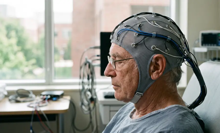
When a neurophysiologist looks at a scrolling EEG trace, they are not looking at raw electrical signals from single points on the scalp. They are looking at differences between paired electrodes, arranged according to a specific plan called a montage.
One of the oldest and most widely taught of these plans is the longitudinal bipolar montage, which strings electrodes together in chains running from the front of the head to the back. This arrangement has shaped how generations of clinicians scan for seizures and slow waves, but its actual diagnostic performance has rarely been tested directly.
What Is a Longitudinal Bipolar Montage?
A longitudinal bipolar montage pairs adjacent electrodes in a line that runs from the front of the skull toward the back, following what is called the parasagittal plane, a strip of scalp that sits roughly parallel to the midline seam of the brain. A typical left-sided chain might link Fp1 to F3, then F3 to C3, then C3 to P3, then P3 to O1, with each pair representing one recording channel.
The visual result is a narrow, vertical “strip” of activity that tracks the long axis of the brain rather than its width. This is deliberate. Because each channel shares one electrode with the channel above it and one with the channel below it, a signal that travels along that anterior-to-posterior line will show up as a linked pattern moving down the page, channel after channel.
The design is meant to make it easier to watch a single electrical event as it spreads across the parasagittal cortex, the strip of brain tissue that runs along either side of the interhemispheric fissure, the deep groove separating the two hemispheres.
How the Longitudinal Bipolar Montage Is Built From the 10-20 System
The chains themselves come from the International 10-20 System, the standardized map of scalp electrode positions used in nearly all clinical EEG recordings.
Electrode names combine a letter for the brain region (Fp for frontopolar, F for frontal, C for central, P for parietal, O for occipital) with a number or letter indicating hemisphere and distance from the midline. Odd numbers sit on the left, even numbers on the right, and “z” marks the midline itself.
From this map, three parasagittal chains are typically built: one running down the left hemisphere, one down the right, and one along the midline through Fz, Cz, and Pz. A true parasagittal chain runs from the frontopolar region straight through frontal, central, and parietal electrodes to the occipital pole, for example Fp1 to F3 to C3 to P3 to O1 on the left side. In routine clinical practice, technologists sometimes substitute a more lateral chain through F7 and T3 instead.
Channel Type | Electrode Pairings | Primary Application |
|---|---|---|
Frontal | Fp1-F3, F3-C3 | Frontal dysrhythmias |
Central | C3-P3, P3-O1 | Localized background |
Temporal | F7-T7, T8-P8 | Temporal lobe focus |
Why Clinicians Favor the Longitudinal Bipolar Montage
The reasoning behind this EEG montage's popularity rests on two claims commonly taught:
The first claim is anatomical alignment. Because the longitudinal chains run parallel to the interhemispheric fissure and the parasagittal convexity, the montage is thought to track discharges that originate or spread along that same front-to-back plane, such as epileptiform activity arising from the mesial frontal or parietal regions. If a discharge travels along a line, a montage built along that same line should show it clearly.
The second claim concerns artifact reduction. Because the electrodes in a longitudinal chain sit farther from the temporalis muscle at the side of the head compared to transverse chains that run left to right through the temporal region, proponents argue that longitudinal montages pick up less muscle-related noise from jaw clenching or facial tension.
Common Artifacts in Parasagittal Chains
Reading any EEG trace requires distinguishing brain signals from artifacts, the noise generated by muscles, eyes, and equipment rather than neurons. Longitudinal bipolar chains produce a recognizable set of artifact patterns:
Eye blinks: large downward deflection at Fp1–F3 and Fp2–F4, diminishing posteriorly
Vertical eye movements: phase reversal at the same frontal pairs
Lateral eye movements: largely absent in chains that omit F7/F8
Frontalis muscle tension: fast, jagged noise focused at Fp1–F3 and Fp2–F4
Sweat or poor electrode contact: slow baseline drift that can mimic delta slowing
Eye blinks generate a large downward deflection at the Fp1–F3 and Fp2–F4 channels, the pairs closest to the eyes, and this deflection shrinks as it moves posteriorly down the chain. Vertical eye movements, such as looking up or down, tend to create a phase reversal at these same frontal pairs, meaning the waveform flips direction between adjacent channels.
Lateral eye movements produce a positive or negative deflection concentrated at F7 or F8 electrodes when those are included in the montage, but a pure parasagittal chain that omits these lateral positions is largely spared from this particular artifact.
Frontalis muscle tension, from frowning or general facial tightness, shows up as fast, jagged noise most visible at the frontal pairs, again Fp1–F3 and Fp2–F4.
A subtler and more clinically dangerous artifact is generalized sweat or poor electrode contact, which produces a slow drifting sway in the baseline that can mimic delta slowing, a genuine slow-wave pattern associated with encephalopathy or other brain dysfunction. This particular artifact matters directly to the evidence discussed next, since mistaking baseline drift for true slowing is exactly the kind of misread error that shows up when reduced-channel recordings are interpreted under time pressure.
The Hairline EEG Study: Testing the Montage Under Pressure
Researchers investigating a rapid screening approach called “hairline EEG” set out to test whether a reduced electrode array, placed near the hairline for speed and convenience, could reliably catch nonconvulsive status epilepticus (NCSE), a state of ongoing seizure activity that lacks the obvious convulsions of a typical seizure and can only be confirmed by EEG. Because NCSE is common in critically ill patients and a full EEG setup takes time, a faster screening method carries real clinical appeal.
The researchers took 120 EEG samples, a mix of normal recordings and various abnormal patterns, and reformatted each one into three separate six-channel montages meant to simulate a hairline recording.
Montage A was a longitudinal bipolar montage covering only limited parasagittal chains.
Montage B used an ear-referential setup measured against the ear on the same side as each electrode.
Montage C used the same referential approach but measured against the ear on the opposite side.
Five trained neurophysiologists then interpreted all three versions, and their readings were compared against the original, full-montage interpretation of the same recordings.
How the Longitudinal Bipolar Montage Performed in the Study
Among the three reduced montages tested, the longitudinal bipolar version performed best, with 71% of samples interpreted correctly. This was close to the ipsilateral ear-referential montage at 70.5%, and both outperformed the contralateral ear-referential montage, which reached only 65%.
But overall accuracy hides important differences depending on what pattern the readers were trying to identify.
Sensitivity for correctly recognizing a normal EEG was high, at 91%, meaning the montage was quite good at confirming when nothing abnormal was present. Sensitivity dropped sharply for seizures, reaching only 72%, with seizure activity frequently mistaken for more reassuring patterns such as a normal trace or generalized slowing.
The weakest result came with periodic lateralized epileptiform discharges (PLEDs), a repeating pattern of sharp waves confined to one side of the brain that often signals significant underlying pathology. Here sensitivity fell to just 54%, meaning nearly half of these discharges went undetected.
The study's authors were direct about the implication: a hairline EEG built on a reduced longitudinal bipolar montage had low sensitivity for detecting seizures, and they explicitly recommended against pursuing hairline EEG as a rapid screening tool for NCSE. The appeal of a faster setup, in other words, did not translate into diagnostic reliability for the conditions it was meant to catch.
Normal EEG sensitivity: 91% (reliably identified)
Seizure sensitivity: 72% (frequently misread as normal or generalized slowing)
PLEDs sensitivity: 54% (nearly half missed)
Conclusion: reduced longitudinal bipolar array is not suitable for rapid NCSE screening
Could a Full Longitudinal Montage Perform Better?
It is tempting to generalize this finding to longitudinal bipolar montages as a category, but the study specifically examined a reduced, six-channel hairline version, not the full 10-20 longitudinal setup used in standard clinical EEG.
Still, the low sensitivity for seizures found here does highlight a broader structural point: any limited-channel longitudinal montage, regardless of its theoretical anatomical advantages, shares the same vulnerability. Fewer electrodes mean less coverage, and less coverage means a higher chance that a discharge occurring outside the recorded strip goes unseen.
How to Read a Longitudinal Bipolar Trace
If you are building familiarity with this montage, a few habits reduce the risk of misinterpretation:
Scan each parasagittal chain from top to bottom looking for a phase reversal, where a waveform points upward in one channel and downward in the adjacent channel that shares a common electrode. This pattern points toward the approximate source of the discharge, since the shared electrode is likely closest to where the abnormal activity originates.
Treat a normal-appearing trace on a reduced longitudinal bipolar recording with caution rather than certainty. The hairline study found that seizures were frequently misread as normal, meaning the absence of obvious abnormality on a limited montage does not rule out genuine seizure activity.
Confirm the specific montage and electrode coverage before drawing a conclusion of “no epileptiform activity.” The overall 71% correct interpretation rate in the study, achieved by trained neurophysiologists, demonstrates that even experienced readers can be misled by incomplete channel coverage.
The Bottom Line on Longitudinal Bipolar Montages
The longitudinal bipolar montage organizes electrodes into parasagittal, front-to-back chains and remains a foundational tool taught throughout clinical neuroscience and neurophysiology training. Its better measurement of parasagittal discharges and reduced contamination from temporal muscle artifacts, are grounded in reasonable anatomical logic.
References
Kolls, B. J., & Husain, A. M. (2007). Assessment of hairline EEG as a screening tool for nonconvulsive status epilepticus. Epilepsia, 48(5), 959-965. https://doi.org/10.1111/j.1528-1167.2007.01078.x
Frequently Asked Questions
What is a longitudinal bipolar montage in EEG?
A longitudinal bipolar montage pairs adjacent electrodes in chains running from the front to the back of the head, following the parasagittal plane. Each channel displays the voltage difference between two neighbors, making it easier to track how electrical activity moves along the brain's long axis.
How is a longitudinal bipolar montage built from the 10-20 system?
It uses standard 10-20 electrode positions to form three chains: left, right, and midline. For example, a left chain typically links Fp1 to F3, then F3 to C3, C3 to P3, and P3 to O1, creating a sequence of bipolar pairs.
Why do clinicians favor the longitudinal bipolar montage?
The chains align with the parasagittal cortex, so discharges spreading front-to-back are thought to appear clearly. Electrodes are also farther from the temporalis muscle, which may reduce muscle-related artifact compared to side-to-side montages.
What common artifacts appear in longitudinal bipolar chains?
Eye blinks produce large downward deflections at the frontal pairs, while vertical eye movements can create a phase reversal there. Frontalis muscle tension shows as fast, jagged noise in the same channels, and poor electrode contact can cause slow baseline drift that mimics pathological slowing.
How should a reader approach a longitudinal bipolar EEG trace?
Scan each chain for a phase reversal, where the waveform flips direction between adjacent channels sharing an electrode, as this points to the likely source. A normal-appearing trace on a reduced montage should be interpreted cautiously, because seizures can be missed when coverage is incomplete.
Emotiv is a neurotechnology leader helping advance neuroscience research through accessible EEG and brain data tools.
Christian Burgos