An electroencephalogram never records a “pure” signal from a single point on the scalp. Every voltage a technologist sees on the screen is the difference between the recording electrode and whatever reference that electrode is compared against.
This single fact is the root of a great deal of confusion for students learning to read EEG traces, because the same underlying brain activity can look strikingly different depending on which reference scheme is chosen.
Among the most commonly used schemes in clinical and research settings is the average montage, sometimes called the common average reference. Learning to recognize what this montage does well, and where it can quietly mislead an inexperienced reader, is one of the more practical skills a first-year student can build.
What Is the Average Montage in EEG?
The average montage compares each electrode's voltage not to a single fixed point, but to the instantaneous mathematical average of every electrode in the recording. At each moment in time, the software adds up the voltages from all active channels, divides by the number of electrodes, and subtracts that average from each individual channel's value.
The intent behind this method is to approximate a neutral, zero-point reference. Because the average is built from the entire electrode array rather than one location, no single site (like an ear or a mastoid) can dominate or distort the picture.
In theory, this allows widespread or diffuse brain activity to appear more symmetrically across the scalp, since no single reference point is pulling the display in one direction.
The montage calculates the instantaneous average of all active electrodes at each moment in time.
This calculated average is then subtracted from every individual channel's voltage.
The goal is a neutral reference, preventing any single physical site from dominating the display.
Setting Up an Average Montage on EEG Equipment
Electrode Placement Considerations
To ensure the mathematical validity of the average, standardized electrode distribution is required. The 10-20 system must be strictly followed to ensure that the global mean remains spatially representative of the head.
Any deviation in placement or electrode impedance can result in a skewed average, leading to inaccurate waveform representations and potential diagnostic errors.
Software Configuration Steps
The digital acquisition software must be set to correctly perform the subtraction of the calculated global mean from each input channel. Technologists need to confirm that the software is reading the full array of sensors to avoid a calculation biased by missing channels.
Once the parameters are set, the display can be toggled in real-time, allowing for efficient review and secondary verification of potential anomalies detected in the raw signals.
Why the Average Montage Can Be Misleading
The average montage has one well-documented weakness that every EEG reader eventually encounters.
Because the reference at every moment is built from all the electrodes combined, a single electrode that records an unusually large voltage spike will pull the entire average toward that value. The mathematical consequence is that every other channel, which is being compared against this newly skewed average, will show a deflection in the opposite direction, even if no real activity occurred there.
This produces a specific and deceptive pattern: a large, sharp discharge at one electrode, paired with smaller, inverted, mirror-image deflections appearing simultaneously across the rest of the scalp. To an inexperienced reader, this can look like a widespread or even bilateral event.
In reality, the source may be entirely focal, confined to the tissue beneath a single electrode, with the rest of the trace only reflecting arithmetic distortion rather than genuine neural activity.
This effect follows directly from how averaging works as a mathematical operation, so it is treated as an established principle in clinical EEG education rather than something that needs to be independently proven in every case. That said, controlled studies directly measuring how often this specific error leads to real diagnostic mistakes are limited. What the available research does confirm is that the average reference is particularly sensitive to two conditions that make this distortion worse: artifact contamination and sparse electrode coverage.
One 2018 simulation study comparing re-referencing techniques found that a related method, the reference electrode standardization technique (a computational approach that estimates a theoretical zero-voltage point), was less affected than the average reference by artifacts mixed into the EEG signal. This means that when a large transient, whether from brain activity or from a non-neural source like a muscle twitch, contaminates the recording, the average reference is comparatively more vulnerable to distortion.
A separate study by Luu et al. looking at stroke-related EEG changes reinforced this concern from a different angle. When researchers took a 128-channel, average-referenced recording and reduced it down to a sparser 32-channel array, the spatial distribution of the abnormal EEG activity became distorted, which the authors noted could result in mislocalization of the affected brain region.
This tells us that the single-discharge distortion problem is not a fixed, constant error. It gets measurably worse when fewer electrodes are covering the scalp, because each remaining electrode carries proportionally more weight in the calculated average.
How to Differentiate Focal from Generalized Activity
Given this vulnerability, the central skill for a student reading an average montage is learning to distinguish a true generalized discharge from a focal event that is simply being smeared across the display by the averaging process. Here’s what you can look for:
Identify the single channel with the largest, sharpest deflection to find the true focal source.
Look for a dipolar field: a clear positive pole and negative pole across the scalp.
Suspect arithmetic distortion when surrounding channels show smaller, simultaneous deflections of the opposite polarity.
A genuinely generalized discharge looks different. All electrodes show a synchronous, symmetrical pattern at roughly the same amplitude, with no clean mirror-image reversal anywhere on the map.
In this case, the average reference is not being pulled in one direction by a single outlier, because every channel is contributing a similarly sized signal to the calculation. The display is, in a sense, more honest here, since the averaging process is not concentrating distortion around one dominant electrode.
When the pattern is ambiguous, cross-checking with a bipolar montage (which displays the voltage difference between adjacent electrode pairs rather than each electrode against an average) is a standard next step. A focal discharge will typically produce a phase reversal, an abrupt flip in the direction of the waveform, at the specific pair of electrodes overlying the affected region. A truly generalized discharge tends to look more diffuse and consistent across multiple adjacent pairs, without a single sharp reversal point.
This differentiation strategy depends heavily on how well the scalp is actually sampled. The stroke-localization study referenced earlier found that accurate description of the spatial distribution of abnormal EEG activity was only achieved with 64-channel or 128-channel recordings. At 32 channels, the distribution became distorted enough to risk mislocalizing the affected region entirely.
For a first-year student, this carries a direct and practical implication: an average montage recorded with a standard clinical setup of 19 to 21 electrodes, the conventional 10-20 system, may carry a higher risk of blurring the line between a true focal abnormality and an artifact of averaging, compared to a high-density array.
Average Montage vs. Referential and Bipolar Displays
Placing the average montage next to its two main alternatives clarifies both its strengths and its blind spots.
A referential montage compares every electrode against one fixed site, commonly the vertex electrode Cz, an earlobe, or the linked mastoids behind the ears. This approach is simple to interpret, but it carries an obvious risk. If that single reference site happens to be contaminated by noise, muscle activity, or even genuine brain activity, that contamination gets subtracted into every single channel on the display.
The average montage was designed partly to avoid this single point of failure. But as the earlier discussion showed, it trades one vulnerability for another. Instead of one bad reference point corrupting the whole recording, one bad electrode's large discharge can now spread distortion across the entire head.
A bipolar montage takes yet another approach, displaying only the voltage difference between neighboring electrode pairs, forming a chain across the scalp. This method is particularly good at highlighting local voltage gradients and phase reversals, which is why it is frequently a go-to choice for localizing focal transients like spikes or sharp waves. Its tradeoff is that it can attenuate or wash out activity that is broad and synchronous across large regions, since neighboring electrodes recording similar signals will show very little difference between them.
The average montage sits between these two, often serving as the default display for viewing the overall topography, or spatial pattern, of rhythmic brain activity, and it is commonly used in quantitative EEG analysis pipelines. But its actual performance is not fixed. It depends heavily on electrode density and the nature of the underlying signal.
Feature | Bipolar Montage | Average Reference Montage |
|---|---|---|
Reference Type | Pairwise subtraction | Global mean extraction |
Sensitivity | Local potential differences | Widespread and focal activity |
Primary Use | Phasing and orientation | Source localization |
This table illustrates how the choice between bipolar and average configurations influences the visualization of neural data, demonstrating that while bipolar setups highlight local activity, the average montage excels at mapping the global topography of electrical events.
What Does Research Say About Average Montages in EEG
The study by Hu et al. comparing re-referencing methods found that a computationally estimated neutral reference was generally superior to the simple average reference across most conditions tested, though the average reference was noted as a reasonable alternative specifically in cases with high sensor noise. This indicates that the average montage is not a universal “best” choice, but rather one option with particular conditions where it performs adequately.
Meanwhile, a separate simulation study by Liu et al. sharpened this picture further. Both the average reference and the computationally estimated reference showed relatively low reconstruction errors compared to a linked-mastoid reference, but their relative performance flipped depending on electrode density.
With a low-density montage, the estimated reference method proved more reliable. With a high-density montage, the average reference actually performed better, unless precise information about electrode positioning was unavailable. The lesson here is that electrode count fundamentally changes which reference method is more trustworthy.
It's worth noting that referential montages are not automatically inferior in every practical setting.
For instance, a study designed by Karakis et al. for critical care environments tested a simplified seven-electrode montage referenced to the vertex electrode Cz, intended for use by residents without dedicated EEG technologists on hand.
This scheme achieved an average sensitivity of 92.5 percent and specificity of 93.5 percent for detecting seizures in intensive care patients. This study did not directly pit the average montage against a referential one in a head-to-head comparison, but it demonstrates that a well-designed referential scheme, applied in the right clinical context, can perform reliably even with a limited number of electrodes, which is a useful counterpoint when weighing montage choices for brain disorders requiring urgent detection, such as nonconvulsive seizures.
Montage Type | Reference Point | Strength | Weakness | Best For |
|---|---|---|---|---|
Average | All electrodes' mean | No single point bias | One bad electrode distorts all | Topography, rhythmic activity |
Referential | Single fixed site | Simple interpretation | Contamination from reference site | Standard clinical use |
Bipolar | Adjacent electrode pairs | Highlights local gradients | Misses broad synchronous activity | Focal transient localization |
Practical Tips for Interpreting an Average Montage
A few habits can help a student avoid the most common misreadings when working with average-referenced data:
Always check the number of electrodes and their scalp coverage before interpreting a pattern. If the recording uses fewer than roughly 32 channels, be cautious about labeling an apparently widespread discharge as truly generalized without further verification.
If a suspicious widespread pattern appears, switch to a bipolar or referential montage and see whether the event resolves into a clear focal maximum. This cross-check is standard practice in clinical reading, though its precise error-reduction rate has not been formally measured in large trials.
Remember that the average montage can generate a false mirror image across every channel. The size of these mirrored deflections scales with the amplitude of the true focal event and scales inversely with the total number of electrodes, meaning fewer electrodes concentrate more distortion into each remaining channel.
The stroke-localization findings showing that 64 channels or more were needed for accurate spatial characterization support a broader rule of thumb: higher electrode density meaningfully improves the reliability of the average montage for localization tasks.
The evidence that the average reference is sensitive to artifact contamination, and that low-density montages tend to favor alternative reference methods, reinforces that the average montage should not automatically be treated as the most robust option when electrode numbers are limited.
Interpreting the Average Montage With Confidence
The average montage remains one of the most widely used re-referencing methods in clinical neuroscience and EEG research, precisely because it offers a reasonably balanced view of brain activity without depending on a single vulnerable reference point. But that balance comes with a specific tradeoff that every reader needs to internalize.
A single large focal discharge can bias the shared average, producing deflections across the entire scalp that mimic a widespread event when the true source is confined to one region.
Reliable differentiation between focal and generalized activity comes down to identifying where the true maximum amplitude sits, checking for the mirror-image pattern that signals arithmetic distortion rather than genuine spread, and confirming ambiguous cases with a bipolar or referential display. The available evidence consistently points to electrode density and head modeling accuracy as the two factors that most strongly determine whether the average montage will give an accurate picture or a distorted one.
Its advantages are clearest in high-density recordings; its limitations become more pronounced in standard clinical arrays with sparser coverage.
References
Hu, S., Lai, Y., Valdes-Sosa, P. A., Bringas-Vega, M. L., & Yao, D. (2018). How do reference montage and electrodes setup affect the measured scalp EEG potentials?. Journal of neural engineering, 15(2), 026013.
Luu, P., Tucker, D. M., Englander, R., Lockfeld, A., Lutsep, H., & Oken, B. (2001). Localizing acute stroke-related eeg changes:: Assessing the effects of spatial undersampling. Journal of clinical Neurophysiology, 18(4), 302-317.
Liu, Q., Balsters, J. H., Baechinger, M., Van der Groen, O., Wenderoth, N., & Mantini, D. (2015). Estimating a neutral reference for electroencephalographic recordings: the importance of using a high-density montage and a realistic head model. Journal of neural engineering, 12(5), 056012. https://doi.org/10.1088/1741-2560/12/5/056012
Karakis, I., Montouris, G. D., Otis, J. A., Douglass, L. M., Jonas, R., Velez-Ruiz, N., ... & Espinosa, P. S. (2010). A quick and reliable EEG montage for the detection of seizures in the critical care setting. Journal of Clinical Neurophysiology, 27(2), 100-105. https://doi.org/10.1097/wnp.0b013e3181d649e4
Frequently Asked Questions
What exactly is an average montage in EEG?
The average montage re-references each electrode’s voltage against the instantaneous mathematical average of all active electrodes. It subtracts this common average from every channel to create a neutral reference point that is not tied to any single scalp location.
Why can the average montage create a misleading pattern of widespread activity?
When one electrode records a large discharge, it pulls the average strongly in its direction. All other channels are then compared to that skewed average, generating mirror-image deflections that look like activity even though only one focal source exists.
How can a student distinguish a true focal discharge from a distorted one on an average montage?
Look for the electrode with the clearly largest amplitude and check for smaller, opposite-polarity signals at the same moment in other channels. A dipolar pattern with one dominant maximum points to a focal event, whereas a true generalized discharge shows synchronous, similarly sized activity everywhere.
What role does electrode density play in the average montage’s reliability?
With fewer electrodes, each channel contributes more weight to the average, so a single large transient distorts the display more severely. Higher-density arrays (e.g., 64 or more channels) reduce this arithmetic artifact and improve the accuracy of spatial localization.
How does the average montage differ from a referential montage?
A referential montage compares every electrode to one fixed physical site, risking contamination if that site is noisy. The average montage avoids a single point of failure but instead can spread distortion from a single focal discharge across the entire scalp display.
When might a bipolar montage be more useful than an average montage?
A bipolar montage displays voltage differences between neighboring electrodes and is excellent for localizing focal transients through sharp phase reversals. It is less helpful for viewing broad, synchronous rhythms, where the average montage often gives a better overview of the overall scalp topography.
What is a practical way to verify a suspicious pattern seen on an average montage?
Switch to a bipolar or referential montage and check whether the apparently widespread event narrows down to a clear focal maximum. This cross-check reveals whether the pattern reflects true generalized activity or is an arithmetic mirror image created by the averaging process.
Is the average montage universally the best reference choice?
No, its performance depends strongly on electrode density and head coverage. In low-density recordings, alternative computational reference methods may be more reliable, while with many channels the average reference often performs well unless precise electrode positions are unknown.
Does the head size of the patient impact the reference calculation?
While the math remains the same, variations in head size necessitate that the electrodes remain proportionally located according to standardized systems to maintain the integrity of the spatial averages being calculated.
Emotiv is a neurotechnology leader helping advance neuroscience research through accessible EEG and brain data tools.
Medical Disclaimer: The information provided on this website is for educational and informational purposes only and is not intended as medical or health advice. This content may contain errors and should not be relied upon to make life-altering health, medical, or lifestyle choices. Always seek the advice of your physician or other qualified health provider with any questions you may have regarding a medical condition or treatment.
Christian Burgos