ניתוח צפיפות זרם מקור (CSD) מעריך היכן זרם חשמלי נכנס או יוצא מרקמה עצבית על ידי בחינת שינויים מרחביים במתח חוץ-תאי. הוא יכול לחדד את הפרשנות של רישומי EEG ומיקרו-אלקטרודות, אך תוקפו תלוי בגיאומטריית האלקטרודות, איכות הדגימה, בחירת הייחוס (רפרנס) והנחות המודל.
What Is Current Source Density?
Current source density describes the distribution of electrical current flowing into and out of a volume of neural tissue. In neuroscience, a source generally represents current leaving the extracellular space, whereas a sink represents current entering it. The terms depend on the chosen sign convention and viewpoint, so a source or sink is best understood as part of a local electrical pattern rather than as a separate anatomical object.
The estimate is usually derived from extracellular voltage measurements collected at multiple nearby positions. Spatial differences between those measurements reveal how rapidly the voltage field changes across tissue. Because the calculation emphasizes local variation, CSD can help distinguish a focal pattern from a broad field produced by activity conducted through surrounding tissue.
CSD does not directly identify a single neuron, synapse, or ion channel. It is a population-level and geometry-dependent estimate of transmembrane current distribution. Within neuroscience, it is therefore used alongside anatomy, electrophysiology, stimulation timing, and behavioral or clinical observations rather than treated as a standalone map of cellular activity.
The Biophysical Basis: From Voltage to Current
When synapses activate, ions flow across the neuronal membrane, generating tiny electrical currents in the surrounding tissue. An extracellular electrode picks up the resulting potential changes, but these changes are a blurred mixture of currents from many cells.
CSD works backward from that recorded voltage to infer the net current entering or leaving the tissue at each point, a picture of where synaptic currents originate and where they return to the cell.
The relationship between the extracellular field potential and the underlying currents is governed by well-established physics, captured in Poisson’s equation. For a conductive medium, the CSD (the net current crossing a small volume) is related to the divergence of the current flow vector, which in turn links to the spatial variation of the field potential.
In a simple, uniform conductor, the CSD is directly proportional to how sharply the voltage changes with distance—mathematically, its second spatial derivative. This insight underpins the classic CSD computation, but real brain tissue rarely behaves like a homogeneous salt bath.
The foundational experiments that established CSD’s biophysical credibility were performed in the frog and toad cerebellum. Researchers measured the full conductivity tensor—a three-dimensional map of how easily current flows in different directions—and found that the tissue was anisotropic (current flowed more readily along certain axes than others) yet remarkably homogeneous (the conductivity did not vary significantly with location) and ohmic (the voltage–current relationship was linear).
Knowing this single conductivity tensor allowed a simplified but physically accurate CSD model, setting the stage for practical applications.
How to Compute Current Source Density
Translating recorded voltages into CSD maps requires careful selection of computational methods. The choice hinges on the complexity of the tissue and the spatial layout of the recording array.
The Classic Second-Spatial-Derivative Method
Under the assumptions of homogeneous and isotropic conductivity, the CSD boils down to a straightforward operation: take the field potential recorded at a series of equally spaced electrode contacts and compute the second derivative along the probe’s axis. In practice, this is done with finite-difference formulas that approximate the derivative using the voltages at neighboring contacts.
However, not all differentiation schemes are equal. A systematic comparison in the anuran cerebellum evaluated different formulas for their accuracy, their tendency to distort rapidly changing spatial patterns (aliasing), and the amount of smoothing they introduce.
Just as choosing the wrong filter can blur a photograph, selecting an inappropriate differentiation scheme can obscure the very events you hope to see. The optimal formula depends on the spatial frequency content of the signals, a lesson reinforced by measuring the spatial energy-density spectrum to find the ideal interelectrode distance.
Beyond the Simplest Assumption: Inverse Methods and Conductivity Profiles
When the tissue is anisotropic or inhomogeneous, the simple second-derivative approach no longer holds. A more general framework starts from Poisson’s equation and incorporates the measured conductivity tensor to reconstruct the true source distribution.
The aforementioned theoretical paper provided the full equations in rectangular Cartesian coordinates, including a rotated coordinate system to align with tilted laminar structures. This foundation allows modern inverse CSD algorithms to correct for directional conductivity and produce more accurate maps.
Crucially, the early demonstration that the cerebellar tissue was homogeneous and ohmic meant that a single, constant conductivity tensor could be used, dramatically simplifying the inverse problem. For many laminated brain regions, this remains a reasonable starting point, though precise corrections for inhomogeneity are sometimes necessary.
Common Algorithms and Assumptions
Several approaches are used, and each makes different demands on the data. Simple finite differences are transparent and work naturally with regularly spaced contacts, while spline-based or kernel-based methods can accommodate broader spatial layouts. In surface EEG, the surface Laplacian transform is a closely related operation that estimates local curvature in the scalp voltage field.
The choice of algorithm should follow the electrode arrangement rather than convenience alone. Common assumptions and decisions include:
Whether conductivity is treated as homogeneous and isotropic.
Whether the recording geometry supports one-, two-, or three-dimensional derivatives.
How boundary conditions and missing channels are handled.
Whether smoothing is applied before spatial differentiation.
After the calculation, the sign convention must be documented clearly, since the visual labels “source” and “sink” can reverse between implementations. Validation can include simulated fields, known stimulus timing, anatomical alignment, and sensitivity analyses using alternative spacing or smoothing parameters. Such checks do not eliminate uncertainty, but they show whether the main pattern is stable.
Tools and Software for CSD Analysis
CSD workflows can be implemented with numerical computing environments, electrophysiology analysis packages, and custom scripts. The core steps usually include importing signals, checking channel locations, filtering with a stated rationale, identifying bad channels or contacts, applying the spatial operator, and visualizing the result alongside the original recording. Software does not remove the need to understand the assumptions built into that operator.
A reproducible workflow keeps acquisition details and transformations separate. The analyst records electrode geometry, reference scheme, conductivity values when used, interpolation method, smoothing parameters, and boundary treatment. Versioned scripts or notebooks can then regenerate figures and support comparisons between algorithms.
A useful implementation should make it possible to inspect intermediate outputs rather than presenting only a final color map. For surface EEG, this includes checking the interpolated voltage field and electrode layout. For microelectrode arrays, it includes confirming contact order, physical spacing, probe orientation, and the treatment of edge contacts. These checks are often more valuable than adding another visualization.
Practical Considerations for Trustworthy CSD Maps
Raw CSD outputs can be misleading if the recording and analysis parameters are not optimized. Three major sources of error can inject spurious sources and sinks:
The spacing between electrode contacts
Electrical noise
Uncertainty about the exact position of the electrodes
Electrode Spacing and Spatial Sampling
The distance between recording sites defines the smallest spatial structure you can faithfully capture. Too large a spacing smooths away fine details and may cause aliasing, where rapid spatial changes masquerade as lower-frequency patterns. Too small a spacing, on the other hand, amplifies the effects of noise, because the second derivative operation is highly sensitive to tiny voltage fluctuations.
The solution is often to measure the spatial energy-density spectrum of the field potential. In the anuran cerebellum, this analysis revealed the frequency bands where the real physiological signal dominated over noise, allowing researchers to choose an interelectrode spacing that maximized true signal capture while minimizing distortion. This empirical optimization transformed a theoretical technique into a practical, high-fidelity tool.
Noise, Electrode Position, and Artifacts
Beyond spacing, three primary error sources can corrupt CSD maps:
Random electrical noise
Uncertainty in the tip position of the recording electrodes
Inaccuracies in the assumed conductivity tensor
In the aforementioned Freeman et al. study, theoretical expressions were derived to estimate the relative magnitude of each error, and experiments confirmed their validity. For example, even a small misalignment between the assumed and actual electrode location could create fake current sink–source pairs.
In the retina, methodological explorations revealed specific scenarios that produced “artifactual source/sinks”. By systematically varying parameters such as referencing, filtering, and electrode array geometry, the researchers identified best practices that led to “minimal variability and noise in the CSD profiles”. This emphasizes that CSD is not a plug-and-play technique, and that careful validation is required to separate genuine physiological events from analysis artifacts.
How Many Spatial Dimensions Are Enough?
A common simplification is to assume that current flows only along the axis of the electrode penetration—a one-dimensional (1D) CSD. This assumption holds when the active neuronal elements are arranged in flat, parallel laminae and the electrode track is perpendicular to them.
In structures like the cortex or cerebellum, where cells are organized in layers, a 1D approximation often suffices. However, if significant currents flow in other directions (as can happen near curved boundaries or with oblique penetrations), a 1D analysis will misattribute volume-conducted signals as local sources.
Applications of CSD Across Neural Systems
The power of CSD becomes evident when it is applied to well-defined circuits. Three classic preparations illustrate how CSD disentangles overlapping signals and reveals the hidden organization of synaptic currents.
Cerebellar Laminar Organisation
The frog and toad cerebellum served as the proving ground for CSD methodology. Applying the optimized technique to vestibulocerebellar input yielded “significantly better temporal and spatial resolution of neuronal events” than raw field potentials alone.
Because the cerebellar cortex is a highly regular laminar structure, CSD maps could pinpoint the layers where synaptic input arrived and where active currents returned, offering a direct readout of the functional connectivity between the vestibular nerve and its target neurons. This work not only validated the method but also demonstrated how CSD could serve as a general tool for laminated brain regions.
Retinal Depth Profiles
The retina, with its well-defined layers, is another ideal tissue for CSD. In the frog retina, a CSD depth profile at the peak of the light-evoked b-wave revealed a large current sink near the outer plexiform layer (OPL), a source at the inner limiting membrane (ILM), and a more complex sequence of events in the inner plexiform layer (IPL).
At light onset, the IPL response unfolded in three orderly steps. An initial sharp sink corresponded to the proximal negative response (PNR), followed by a slower source that mirrored the b-wave, and finally an even slower sink with the time course of the M-wave.
This decomposition is impossible from a single voltage trace, where these components merge into a single waveform. The OPL sink was clearly tied to the b-wave generators, while the M-wave sink appeared small because it partly canceled with the overlapping b-wave source at the same depth.
CSD thus provided a layer-by-layer dissection of the retinal circuit’s response to light, separating the contributions of distinct cell populations.
Cortical Laminar Profiles
Perhaps the most striking demonstrations of CSD’s value come from studies of the primate neocortex. In macaque primary visual (V1), auditory, and somatosensory areas, laminar LFP recordings were analyzed with CSD to localize the generators of α-band oscillations. The CSD maps revealed α current generators in all cortical layers—supragranular, granular, and infragranular—with the strongest sources in the superficial supragranular layers.
This finding corrected a long-standing misinterpretation. The raw LFP signal showed maximal α power in the deep infragranular layers, but CSD made clear that this was an illusion caused by “contamination of the infragranular LFP signal by activity that is volume-conducted from the stronger supragranular α generators”.
Volume conduction, where currents spread passively through the tissue, smears the true origins of the signal. CSD filters out this smearing, revealing that the α rhythm is not a deep-layer monopoly but a multi-laminar phenomenon that likely participates in both feedforward and feedback processing.
A second cortical study used a band-limited CSD power analysis to dissect the laminar profile of visual responses in V1. When a stimulus appears abruptly, the LFP shows a sharp transient followed by a sustained component. By separating phase-locked (trial-averaged) and non-phase-locked (trial-by-trial power) contributions, the CSD analysis found a short-latency current sink in layer 4C—the classic thalamocortical input—and, about 500 µm deeper, a distinct sustained sink that persisted for as long as the visual stimulus remained on the screen.
The deeper sink was non-phase-locked, meaning its timing varied from trial to trial, and likely represents recurrent or feedback processing rather than the initial feedforward drive. This dissociation between initial detection and sustained representation would be completely invisible in a standard LFP average, underscoring CSD’s unique ability to reveal the temporal architecture of cortical processing.
System | Key Finding | CSD Advantage |
|---|---|---|
Cerebellum | Resolved laminar synaptic input | Better spatial resolution |
Retina | Dissected b-wave components | Layer-by-layer analysis |
Cortex | Corrected α generator location | Revealed volume conduction |
Interpreting CSD in the Context of Neuronal Activity
CSD maps are sometimes criticized as mathematical abstractions detached from spiking activity. However, the collected evidence refutes this since CSD sinks and sources are tightly coupled to neuronal firing.
Linking CSD to Spiking and Excitability
In the α-rhythm study by Haegens et al., multiunit activity (MUA) recorded simultaneously with the LFP was phase-locked to the local current source/sink configurations detected by CSD. This means that when CSD showed a strong current sink in a given layer, nearby neurons were more likely to fire action potentials at that phase of the oscillation.
The coupling confirms that “α rhythms index local neuronal excitability fluctuations” and that CSD sinks correspond to net excitatory synaptic drive. This empirical grounding gives CSD its biological meaning as it pinpoints the lamina where synaptic drives and active membrane processes are strongest, not just the passive volume-conducted echoes.
Distinguishing Different Dynamics with CSD
The visual response study by Maier et al. provided another layer of insight. The same V1 microcircuit generated two fundamentally different CSD patterns for a simple visual stimulus. The early, phase-locked sink in layer 4C reflects the precisely timed arrival of thalamic input. The later, non-phase-locked sink, centered deeper, is consistent with sustained intracortical processing that does not lock to stimulus onset.
CSD thus can dissect a single gross LFP waveform into components that arise from distinct neural mechanisms—feedforward versus recurrent, transient versus sustained—revealing a richer picture of circuit dynamics than the raw voltage signal ever could.
Why Current Source Density Analysis is a Crucial Tool for Neuroscientists
Current source density analysis moves beyond recording what the electrode merely “hears” to constructing a physical picture of the currents that generate that signal. By integrating rigorous biophysical theory with careful experimental optimization and innovative analysis variants, CSD uncovers the hidden laminar choreography of synapses and active currents.
Whether mapping retinal circuits, cerebellar inputs, or cortical rhythms, CSD consistently resolves details that conventional field potentials blur: it separates volume-conducted signals from local activity, disentangles overlapping synaptic events, and reveals the true spatial origin of sustained and oscillatory processing.
For any neuroscientist working with laminar probes or cortical imaging data, CSD is not a dispensable add-on but a foundational step toward an honest interpretation of extracellular recordings. It transforms ambiguous voltage traces into a transparent map of where and when neurons exchange information, making it a cornerstone technique for understanding how neural circuits operate.
CSD vs Raw EEG Signals: Why It Matters
Raw EEG displays voltage relative to a reference, whereas CSD displays a spatial derivative of that voltage field. Raw signals preserve broad field information and are useful for assessing global synchronization, event timing, and overall data quality. CSD suppresses some spatially smooth activity and highlights local curvature, which can make a focal pattern easier to see.
The distinction is not simply between an inferior and a superior signal. A spatial derivative changes the question being asked. A broad potential may be biologically meaningful even if CSD attenuates it, while a sharp CSD feature may reflect sparse sampling, interpolation, or noise if the measurement geometry is weak.
The practical comparison is clearest when the two representations are inspected together. A feature that remains spatially and temporally consistent across raw and transformed data is easier to interpret than one that appears only after aggressive filtering. CSD can provide greater spatial specificity, but that specificity must be weighed against the information removed by differentiation.
How Current Source Density Analysis Turns Voltage Traces into Trustworthy Maps of Brain Signaling
Current source density analysis shifts the focus from the raw voltage an electrode hears to the physical locations where neurons actually exchange electrical signals. By filtering out the blur of volume conduction, this technique corrects illusions in standard recordings, such as alpha activity appearing strongest where it is only passively echoed. Across cerebellar, retinal, and cortical circuits, it consistently separates incoming drivers from sustained processing, exposing the layer-by-layer activity that ordinary traces merge together.
Yet CSD is not an automatic fix; its reliability depends on careful electrode spacing, noise control, and proper interpretation. The method links best to real neuron firing when sinks and sources align with spiking activity, giving scientists a trustworthy map of neural communication. This is crucial because knowing where and when circuits exchange information is essential for making honest sense of brain recordings.
References
Nicholson, C., & Freeman, J. A. (1975). Theory of current source-density analysis and determination of conductivity tensor for anuran cerebellum. Journal of neurophysiology, 38(2), 356-368. https://doi.org/10.1152/jn.1975.38.2.356
Freeman, J. A., & Nicholson, C. H. (1975). Experimental optimization of current source-density technique for anuran cerebellum. Journal of neurophysiology, 38(2), 369-382. https://doi.org/10.1152/jn.1975.38.2.369
Xu, X. I. J. I. N. G., & Karwoski, C. J. (1994). Current source density (CSD) analysis of retinal field potentials. I. Methodological considerations and depth profiles. Journal of neurophysiology, 72(1), 84-95. https://doi.org/10.1152/jn.1994.72.1.84
Haegens, S., Barczak, A., Musacchia, G., Lipton, M. L., Mehta, A. D., Lakatos, P., & Schroeder, C. E. (2015). Laminar profile and physiology of the α rhythm in primary visual, auditory, and somatosensory regions of neocortex. The Journal of Neuroscience, 35(42), 14341-14352. https://doi.org/10.1523/JNEUROSCI.0600-15.2015
Maier, A., Aura, C. J., & Leopold, D. A. (2011). Infragranular sources of sustained local field potential responses in macaque primary visual cortex. The Journal of Neuroscience, 31(6), 1971-1980. https://doi.org/10.1523/JNEUROSCI.5300-09.2011
Frequently Asked Questions
What is Current Source Density (CSD) analysis and what does it reveal about brain activity?
CSD analysis transforms extracellular voltage recordings into maps of where current enters (sinks) and leaves (sources) neurons, revealing the laminar location and timing of synaptic activity. It provides superior resolution of neuronal events compared to conventional field-potential analysis, allowing researchers to pinpoint the precise layers where neural computations unfold.
How does CSD analysis work from a biophysical perspective?
When synapses activate, ions flow across neuronal membranes, generating tiny electrical currents in surrounding tissue, which an extracellular electrode records as a blurred mixture from many cells. CSD works backward from that recorded voltage, using Poisson’s equation and the spatial variation of the field potential, to infer the net current entering or leaving tissue at each point—essentially taking the second spatial derivative of the voltage in a simple uniform conductor.
Why is CSD analysis considered better than standard field-potential analysis?
Standard LFP recordings contain overlapping contributions from many sources, making it difficult to identify where signals originate. CSD filters out volume-conducted signals and disentangles overlapping synaptic events, revealing the true spatial origin of activity, such as distinguishing between feedforward and feedback processing in cortical layers.
What are the practical requirements for obtaining trustworthy CSD maps?
Three major sources of error can corrupt CSD maps: electrode spacing (too large causes aliasing, too small amplifies noise), electrical noise, and uncertainty in electrode position or assumed conductivity. The optimal solution involves measuring the spatial energy-density spectrum to choose an interelectrode spacing that maximizes true signal capture while minimizing distortion.
When is a 1D CSD analysis sufficient, and when is it not?
A 1D CSD analysis assumes current flows only along the axis of electrode penetration, which holds when active neuronal elements are arranged in flat, parallel laminae and the electrode track is perpendicular to them, as in cortex or cerebellum. However, if significant currents flow in other directions, such as near curved boundaries or with oblique penetrations, 1D analysis will misattribute volume-conducted signals as local sources.
What are the main applications of CSD analysis across different brain regions?
CSD has been applied to the cerebellum to map vestibulocerebellar inputs, to the retina to dissect light-evoked responses layer by layer (e.g., separating b-wave, PNR, and M-wave components), and to the neocortex to localize alpha generators and visual responses. In each case, CSD provides a layer-by-layer dissection of synaptic currents that standard voltage traces blur together.
Why is CSD considered a foundational step for honest interpretation of extracellular recordings?
CSD transforms ambiguous voltage traces into a transparent map of where and when neurons exchange information, separating volume-conducted signals from local activity and disentangling overlapping synaptic events. It is not a dispensable add-on but a crucial tool for understanding how neural circuits operate, especially for researchers using laminar probes or cortical imaging data.
What is the difference between a current source and a current sink?
A source is conventionally associated with current leaving the extracellular space, while a sink is associated with current entering it. The labels depend on sign convention and viewpoint.
Can CSD be used with EEG?
Yes. EEG CSD commonly uses a surface Laplacian-like transformation to emphasize local scalp-field differences and reduce some effects of broad volume conduction.
What are the main limitations of CSD?
Important limitations include sparse or irregular electrode layouts, noise amplification, uncertain conductivity, edge effects, imperfect interpolation, and ambiguity about the underlying anatomical generator.
Emotiv היא מובילה בתחום הנוירוטכנולוגיה המסייעת לקדם מחקר במדעי המוח באמצעות כלי EEG נגישים וכלי נתוני מוח.
כריסטיאן בורגוס